 |
 |
 |
 | Wave-equation inversion of time-lapse seismic data sets |  |
![[pdf]](icons/pdf.png) |
Next: Joint Inversion of Multiple
Up: APPENDIX A
Previous: APPENDIX A
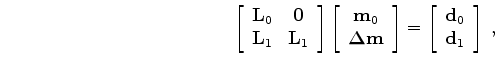
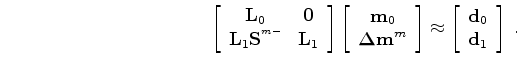
We can formulate baseline and monitor data modeling as follows:
![\begin{displaymath}\begin{array}{ccc} \left [ \begin{array}{cc} {\bf L}_{0} & {\...
... {\bf d}_{0} \\ {\bf d}_{1}\\ \end{array} \right ] \end{array},\end{displaymath}](img57.png) |
(A-1) |
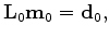
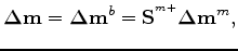
which can be divided into the following two parts:
 |
(A-2) |
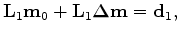
 |
(A-3) |
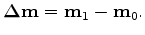
where the time-lapse reflectivity image
 is given by
 |
(A-4) |
Note that Equation A-1 assumes that both
 and
and
 are collocated.
This means that there is no physical movement of the reflector between the baseline and the monitor images.
In addition, equation A-1 assumes that there are no overburden velocity changes.
If stress changes cause any physical movement of a point from baseline position
are collocated.
This means that there is no physical movement of the reflector between the baseline and the monitor images.
In addition, equation A-1 assumes that there are no overburden velocity changes.
If stress changes cause any physical movement of a point from baseline position
 in
to monitor position
in
to monitor position
 in
, we can update equation A-3 such that the point in
is repositioned at
.
The updated modeling equation for the monitor data then becomes
in
, we can update equation A-3 such that the point in
is repositioned at
.
The updated modeling equation for the monitor data then becomes
 |
(A-5) |
where
 is an orthogonal warping operator that aligns
to
, and
is an orthogonal warping operator that aligns
to
, and
 |
(A-6) |
is the time-lapse image estimated at the monitor position
.
And the combined modeling equation becomes
![\begin{displaymath}\begin{array}{ccc} \left [ \begin{array}{cc} {\bf L}_{0} & {\...
... {\bf d}_{0} \\ {\bf d}_{1}\\ \end{array} \right ] \end{array}.\end{displaymath}](img69.png) |
(A-7) |
However, note that equation A-7 requires that we know the true reflector position in the monitor which we may obtain from a geomechanical model.
Furthermore, any regularization on the time-lapse image must be applied at the monitor position, or by first repositioning the time-lapse image to the baseline position as follows:
 |
(A-8) |
where
 is the time-lapse image at the baseline position and
 is an operator that repositions events from the monitor position to the baseline position.
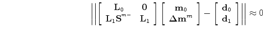
Assuming we migrate the monitor data with the true monitor velocity, we arrive at the image-space inversion problem by minimizing the quadratic-norm
![\begin{displaymath}\begin{array}{ccc} \left \vert\left\vert \left [ \begin{array...
...array} \right ] \right \vert \right \vert \approx 0 \end{array}\end{displaymath}](img73.png) |
(A-9) |
for which the solutions
 and
and
 satisfy the solution
![\begin{displaymath}\begin{array}{ccc} \left [ \begin{array}{cc} {\bf L}_{0}^{T}{...
... {\bf d}_{0} \\ {\bf d}_{1}\\ \end{array} \right ] \end{array},\end{displaymath}](img76.png) |
(A-10) |
or simply
![\begin{displaymath}\begin{array}{ccc} \left [ \begin{array}{cc} {\bf H}_{0}+{\bf...
...de m}_{1}\\ {\bf\tilde m}_{1} \end{array} \right ] \end{array}.\end{displaymath}](img77.png) |
(A-11) |
Note that the time-lapse image we obtain is
at the monitor position and not
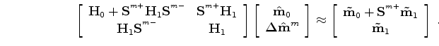 at the baseline position.
Although what is most interesting is
, as shown later in this section, we may choose to re-write the formulation as a function of
at the baseline position.
Although what is most interesting is
, as shown later in this section, we may choose to re-write the formulation as a function of
 .
.
Assuming we migrate the monitor data with the wrong (e.g. baseline) velocity, then equation A-10 becomes
![\begin{displaymath}\begin{array}{ccc} \left [ \begin{array}{cc} {\bf L}_{0}^{T}{...
...{\bf d}_{0} \\ {\bf d}_{1} \\ \end{array} \right ] \end{array},\end{displaymath}](img80.png) |
(A-12) |
where
 , the migration operator with the monitor geometry but with baseline velocity migrates the monitor data to apparent position
 , and
, and
 repositions the migrated data from
to
.
However, because the operator
repositions the migrated data from
to
.
However, because the operator
 is a function of the true monitor velocity, if the true monitor velocity is known, we should solve equation A-11 instead of equation A-12.
Note that in the case where the monitor migration velocity is the correct one, equation A-12 becomes equation A-11.
If we have neither the true monitor velocity nor a geomechanical model, we may modify the Hessian in equation A-12 using the apparent displacements
between
and
so we can approximate equation A-12 as
is a function of the true monitor velocity, if the true monitor velocity is known, we should solve equation A-11 instead of equation A-12.
Note that in the case where the monitor migration velocity is the correct one, equation A-12 becomes equation A-11.
If we have neither the true monitor velocity nor a geomechanical model, we may modify the Hessian in equation A-12 using the apparent displacements
between
and
so we can approximate equation A-12 as
|
(A-13) |
Then equation A-11 becomes
![\begin{displaymath}\begin{array}{ccc} \left [ \begin{array}{cc} {\bf H}_{0}+{\bf...
...}_{1}\\ {\bf\tilde m}^{a}_{1} \end{array} \right ] \end{array},\end{displaymath}](img85.png) |
(A-14) |
where
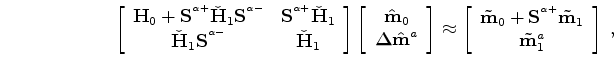 is the modified Hessian in which we account for the mis-positioning due to compaction and velocity change.
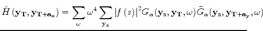
To account for such mis-positioning, we compute the updated Hessian using perturbed Green's functions:
is the modified Hessian in which we account for the mis-positioning due to compaction and velocity change.
To account for such mis-positioning, we compute the updated Hessian using perturbed Green's functions:
 |
|
|
|
 |
|
|
(A-15) |
where 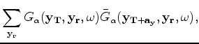 denotes an apparent point in the monitor image that corresponds to baseline point
 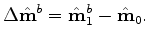 .
The modified Green's function
.
The modified Green's function
 is given by
 |
(A-16) |
where
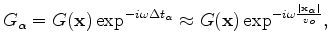 is the time-delay corresponding to the absolute apparent displacement
 and
and  is the baseline velocity.
Instead of inverting for the time-lapse image at the monitor position, another approach is to directly invert for
 at the baseline position by making the substitution
 |
(A-17) |
into equation A-9 to obtain
![\begin{displaymath}\begin{array}{ccc} <tex2html_comment_mark>32 \left [ \begin{a...
...} {\bf d}_{0} \\ {\bf d}_{1}\\ \end{array} \right ] \end{array}\end{displaymath}](img97.png) |
(A-18) |
which leads to the image-space problem
![\begin{displaymath}\begin{array}{ccc} \left [ \begin{array}{cc} {\bf H}_{0}+{\bf...
...}_{1}\\ {\bf\tilde m}^{b}_{1} \end{array} \right ] \end{array}.\end{displaymath}](img98.png) |
(A-19) |
where
 , the migrated monitor image repositioned to the baseline position
, is defined as
, the migrated monitor image repositioned to the baseline position
, is defined as
 |
(A-20) |
If we migrate the monitor data with the baseline velocity, equation A-19 becomes
![\begin{displaymath}\begin{array}{ccc} \left [ \begin{array}{cc} {\bf H}_{0}+{\bf...
...}_{1}\\ {\bf\tilde m}^{b}_{1} \end{array} \right ] \end{array},\end{displaymath}](img101.png) |
(A-21) |
where,
 |
(A-22) |
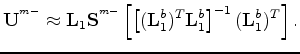
However, provided the velocity change is isotropic, compaction effects are small, differences in kinematics are small, and the velocity change is small, we can make the following approximation:
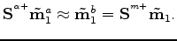 |
(A-23) |
where the operator
is a function of both the monitor velocity and geometry, whereas
 is a function of the baseline velocity but the monitor geometry.
 is an orthogonal operator that translates a data due to a reflectivity spike at baseline position
and baseline background velocity
is an orthogonal operator that translates a data due to a reflectivity spike at baseline position
and baseline background velocity  , to data due to a spike at
and monitor background velocity
, to data due to a spike at
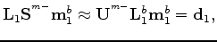
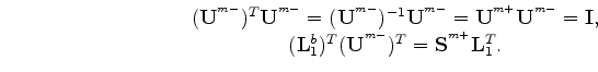
and monitor background velocity  . Note that in equation A-23, we have made the following approximation
![$\displaystyle {\bf U}^{^{m-}}\approx {\bf L}_{1} {\bf S}^{^{m-}}\left[ \left[({\bf L}^{b}_{1})^{T}{\bf L}^{b}_{1}\right]^{-1}({\bf L}^{b}_{1})^{T}\right].$](img108.png) |
(A-24) |
Provided equation A-23 holds, we can write
 |
(A-25) |
where,
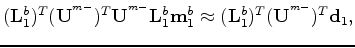 |
(A-26) |
Therefore, we can write
 |
(A-27) |
where,
 is the Hessian computed using the baseline velocity but with the monitor geometry.
Making these substitutions into equation A-19, we have
is the Hessian computed using the baseline velocity but with the monitor geometry.
Making these substitutions into equation A-19, we have
![\begin{displaymath}\begin{array}{ccc} \left [ \begin{array}{cc} {\bf H}_{0}+{\bf...
...}_{1}\\ {\bf\tilde m}^{b}_{1} \end{array} \right ]. \end{array}\end{displaymath}](img113.png) |
(A-28) |
An important advantage of the formulation in equation A-28 is that it allows us to readily regularize the time-lapse image.
However, it may be desirable to invert directly for the individual seismic images, as shown in the following sections.
|
|
|
|
| Wave-equation inversion of time-lapse seismic data sets | |
|
Next: Joint Inversion of Multiple
Up: APPENDIX A
Previous: APPENDIX A
2011-05-24