Anisotropic tomography with rock physics constraints

Numerical tests

We design a walkaway VSP survey on a 2D study area shown in Figure 2. There are 51 sources distributed evenly along a 5 km line on the surface with 2.5 km maximum offset, and 10 receivers fixed every 1 km down the borehole. This acquisition geometry is designed to be similar to the industry standard VSP surveys, which have good constraints for vertical velocity and $\delta$ , but fewer constraints for $\epsilon$ in the deeper part due to the limited propagation angles.

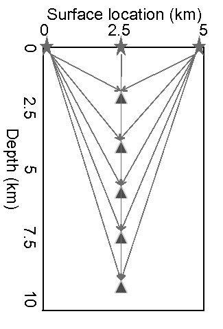
AcquiGeo Figure 2. Walkaway VSP acquisition geometry.

Two 1.5D models are evaluated using this method. One is a shale (sandy shale) model which completely follows the covariance matrix we generated from the rock physics modeling; the other is the same except for a layer of isotropic sand where the prior information is ``wrong''.

Now we are ready to test our method using different prior information. For different tests, we apply the same smoothing operator $\mathbf{S}$ , but different estimates of point-by-point cross-parameter covariance $\mathbf{\sigma}$ . In the notations below, ``no prior'' means $\mathbf{\sigma} = \mathbf{I}$ ; ``column weighting'' means $\mathbf{\sigma}$ has only diagonal elements which are constant for every grid point in the subsurface; ``diagonal covariance'' means $\mathbf{\sigma}$ has only diagonal elements which vary according to the rock physics modeling results; ``full covariance'' means $\mathbf{\sigma}$ has all nine elements which vary according to the rock physics prior for each grid point in the subsurface.

model1
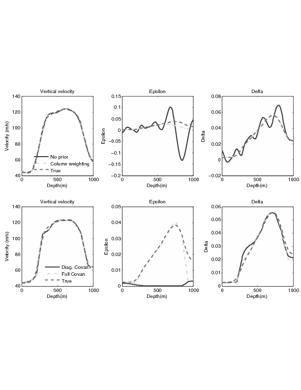
Figure 3. Inversion results of the shale (sandy shale) model. Panels on the left show the velocity perturbation, in the middle $\epsilon$ perturbation, and on the right $\delta$ perturbation. The top row shows the inversion results without rock physics prior knowledge: Solid line: No prior; Dashed dot line: Column weighting; Dashed line: True model. The bottom row shows the inversion results with some rock physics knowledge: Solid line: Diagonal covariance; Dashed dot line: Full covariance; Dashed line: True model.

Figure 3 shows the inversion results of the shale (sandy shale) model. It is obvious that vertical velocity is the best constrained variable, therefore, all inversion schemes yield good estimations for vertical velocity. However, instability is seen in the results of $\epsilon$ and $\delta$ when no prior information is included. The oscillations in $\epsilon$ and $\delta$ are out-of-phase, which is the numerical proof for the theoretical predicted trade-off between these two parameters. Inversion with column weighting yields more stable results for $\delta$ and the shallow part of $\epsilon$ . For the deeper part and also less constrained part of $\epsilon$ , column weighting gives a less satisfactory result. When rock physics prior knowledge is introduced, the inversion is further stabilized. Both the diagonal and the full covariance give good estimations for velocity and $\delta$ , while superior result for $\epsilon$ is obtained by full covariance since correct prior knowledge adds information to the inversion. The fact that a much closer estimation for $\epsilon$ was produced using full covariance rather than the diagonal one suggests that large cross-terms exist in the covariance matrix.

model2
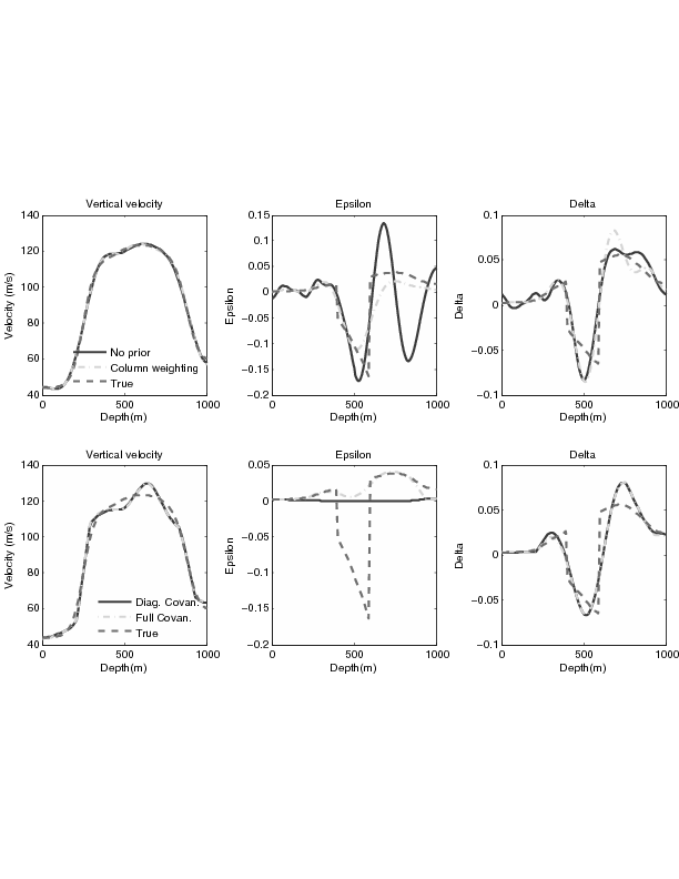
Figure 4. Inversion results of the shale model with an isotropic sand layer. Panels are arranged in the same order as Figure 3.

Figure 4 shows the inversion results of the shale (sandy shale) model with an isotropic layer in the middle. Similar stability conclusions can be drawn as for the shale (sandy shale) case. Notice that for the well-constrained variable $\delta$ , inversion is able to resolve the isotropic layer even though ``wrong'' prior information is provided. However, the inversion result is highly biased towards the prior information for $\epsilon$ where it is not so well constrained.

Anisotropic tomography with rock physics constraints