Residual-moveout analysis in presence of strong lateral velocity anomalies

Residual moveout analysis

Starting from the images shown in the previous section, I performed a conventional residual moveout analysis by applying the following angle-domain moveout

$$\Delta z = \left(1-\rho\right) \tan^2 \gamma,$$ (1)

over a range of values for $\rho$ , and then computing the stack power from the moved-out ADCIGs. For constant velocity errors in the half space above the reflector, the parameter $\rho$ is approximately related to the ratio between the current migration slowness $s_{\rm mig}$ and the true slowness $s$ ; that is, $\rho \approx s_{\rm mig}/s$ (Biondi and Symes, 2004).

Avg-Power-all-0-overn
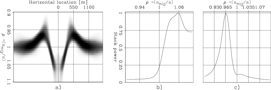
Figure 5. (a) Stack power as a function of horizontal location X and the moveout parameter $\rho$ , corresponding to the full-bandwidth image shown in Figure 3. Graphs of the function in panel a) at (b) X=0 km, and (c) X=.55 km.

Figure 5a shows the stack power as a function of horizontal location X and moveout parameter $\rho$ , averaged over the depth interval of the reflector. The panels in Figure 5b and 5c show the graphs of this function at (b) X= 0 km and (c) X=.55 km.

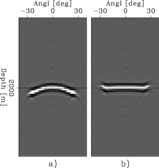
In the middle of the reflector the residual moveout is not well described by a one parameter curve, and thus in Figure 5b the stack power peak is broad and not well defined. Figure 6 shows the central ADCIG before (a) and after (b) residual moveout with $\rho$ =1.06. Whereas the power of the stack is maximum for $\rho$ =1.06 (see Figure 5b), the gather shown in Figure 6b is far from being flat.

In contrast, at X=.55 km, the residual moveout is well described by a one-parameter curve and the stack power peak is sharp and well defined in Figure 5c. However, at $\rho =1$ the stack power curve is almost flat. If we relied on the numerical derivative of this curve to compute the velocity gradient, we might be relying on the wrong information. The power of the stack is maximum for $\rho$ =.965 (see Figure 5c) and indeed the ADCIG moved-out with this value of $\rho$ is flat, as shown in Figure 7b.

Rmo-all-X0-overn Figure 6. ADCIGs at X=0 km before (a) and after (b) residual moveout with $\rho$ =1.06.

Rmo-all-X550-overn Figure 7. ADCIGs at X=.55 km before (a) and after (b) residual moveout with $\rho$ =.965.

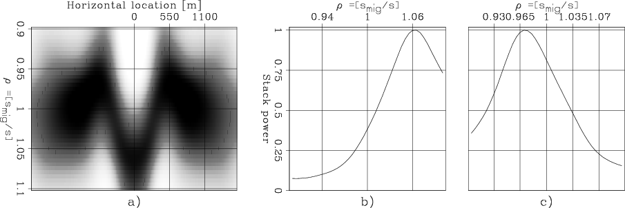
A simple solution to the problems identified above could be to image only the low frequency component of the data. Figure 8 shows the stack-power function when computed from the low-frequency image shown in Figure 4. In this case the stack-power peaks are well defined at both X=0 km and X=.55 km, and they are sufficiently broad that the derivative of the stack-power with respect to $\rho$ , evaluated at $\rho =1$ , would provide useful information for the computation of the velocity gradient.

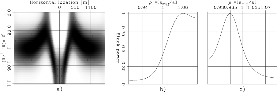
However, seismic data are not always available with sufficient signal-to-noise ratio at low frequencies. In these cases, the challenge can be tackled by smoothing the stack-power function along the moveout parameter before evaluating the derivatives. Figure 9 shows the stack-power function when computed from the full-bandwidth image and then smoothed along the $\rho$ axis. This function has many similarities to the low-frequency one shown in Figure 8, but does not require data with good signal-to-noise ratio at low frequencies.

Avg-Power-all-0-VLowFreq-overn
Figure 8. (a) Stack power as a function of horizontal location and moveout parameter $\rho$ corresponding to the low-passed image shown in Figure 4. Graphs of the function in panel a) at (b) X=0 km, and (c) X=.55 km.

Smooth-Power-all-0-overn
Figure 9. (a) Stack-power function resulting from smoothing along the $\rho$ axis the function shown in Figure 5. Graphs of the function in panel a) at (b) X=0 km, and (c) X=.55 km.

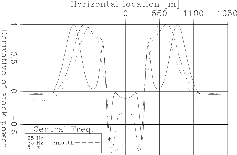
Finally, Figure 10 shows the derivatives of the stack-power functions shown in the previous three figures, evaluated numerically at $\rho =1$ . These functions would be the starting data from which the velocity gradient is computed in a wave-equation migration velocity analysis method (Biondi, 2010,2008; Zhang and Biondi, 2011). The solid line, which corresponds to the full-bandwidth data without smoothing, would provide misleading information and possibly would prevent proper convergence of the velocity estimation algorithm. On the contrary, both the curve computed from the low-frequency data (dotted line) and the one obtained by smoothing the stack-power along $\rho$ (dashed line) would provide useful information for the computation of the gradient.

Der-Power-all-overn
Figure 10. Derivatives of the stack-power functions evaluated numerically at $\rho =1$ : solid line - full-bandwidth data (Figure 5), dashed line - full-bandwidth data with smoothing (Figure 9), dotted line - low-passed data (Figure 8).

Residual-moveout analysis in presence of strong lateral velocity anomalies