Implicit finite difference in time-space domain with the helix transform

Formulation for 1 dimension

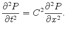
The two-way acoustic wave equation in one dimension reads:

$$\frac{\partial^2 P}{\partial t^2} = C^2 \frac{\partial^2 P}{\partial x^2}.$$ (7)

In order to formulate it as an implicit finite-difference approximation, I first looked to the formulation of the implicit finite-difference operator of the 1-way wave equation in frequency-space domain in Claerbout (2009) Chapter 9. The Crank-Nicolson differencing method is used to create an implicit finite-difference approximation for downward-continuation of a wavefield:

$$\frac{P^x_{z+1} - P^x_z}{\Delta z} = \frac{v}{-i \omega 2} \left(... ...^2} + \frac{P^{x+1}_{z+1} - 2P^x_{z+1} + P^{x-1}_{z+1}}{2 \Delta z^2} \right) .$$ (8)

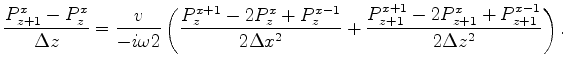The Crank-Nicolson method achieves better accuracy by balancing the 2nd derivative between the current wavefield values (at depth $z$ ) and at the next as-of-yet unknown wavefield values (at depth $z+1$ ). Hence the division by $2$ in the denominators of Equation 8. Borrowing from this methodology, I attempted to formulate a scheme which balances the values of the wavefield at known and unknown locations. Since Equation 7 has a second derivative on the left hand side (as opposed to first derivative in Equation 8), it implies that this balancing must be done over three time ``locations''. In one dimension, these considerations led me to the following approximation:

$$\frac{P^{t+1}_x -2P^t_x + P^{t-1}_x}{\Delta t^2} = \frac{C^2}{3 \... ...1} \right) + \left( P^{t-1}_{x+1} - 2P^{t-1}_x + P^{t-1}_{x-1} \right) \right].$$ (9)

Note that the division by $3$ effectively averages the spatial derivative between the three time steps: $t-1$ , $t$ and $t+1$ . In order to propagate the wavefield, the values of the the wavefield at time $t+1$ must be equated to the values at times $t$ and $t-1$ .

Implicit finite difference in time-space domain with the helix transform