Implicit finite difference in time-space domain with the helix transform

Introduction

Implicit finite difference is a widely used method in geophysical data processing, commonly utilized for the approximation of the differential wave equation when extrapolating wavefields. In comparison with explicit methods, implicit finite difference has unconditional numerical stability, thus enabling larger finite differencing steps during the computation. This is an attractive prospect, as the implication is a shorter processing time for wave extrapolation. However, implementing implicit finite difference in a multidimensional problem is not trivial. The method requires the solution of a sparse set of linear equations per each propagation step. The cost of solving these linear equations, and the computational complexity required, becomes unreasonable at anything greater than 2 dimensions. It is possible to split the solver so that only one dimension of the problem is computed at each propagation step, thus reducing the complexity and possibly the amount of resources required for the computation. However, this method may introduce azimuthal anisotropy to the solution if the actual differential equation being solved is non-separable.

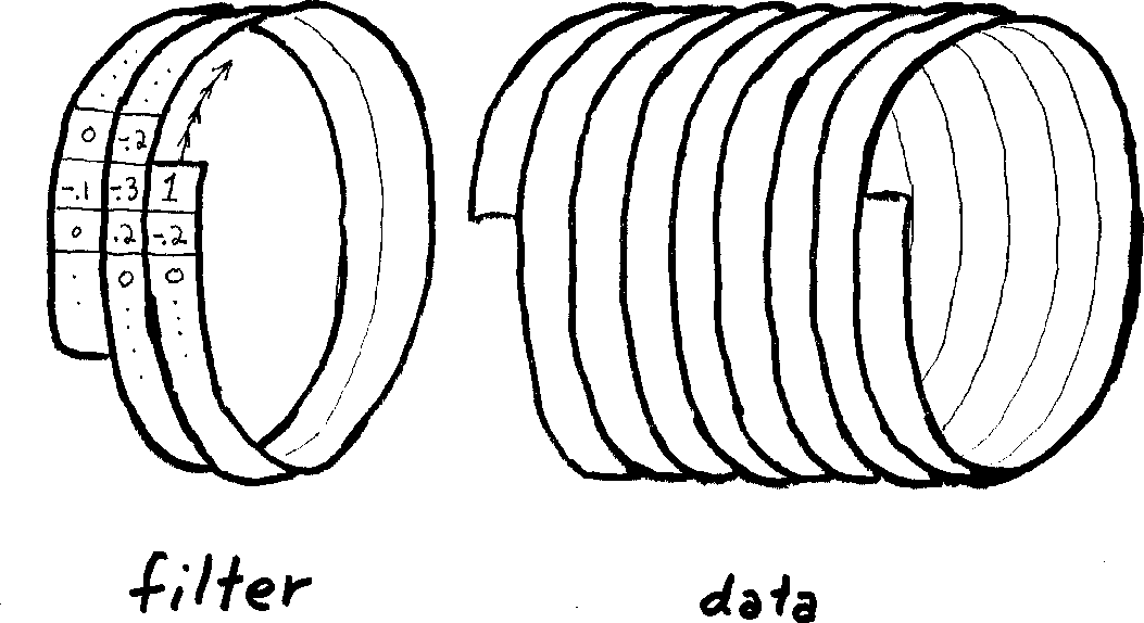
Two concepts combine to greatly aid us in this matter. The first is the helix approach, envisaged in Claerbout (1997). The helix effectively enables us to treat multidimensional problems as one dimensional problems. Specifically, it enables execution of multidimensional convolutions as 1-D convolutions, and likewise for deconvolutions. Convolution equates to polynomial multiplication, while deconvolution equates to polynomial division. The application of convolution or deconvolution to a data set is likened by Claerbout to winding a coil (the filter coefficients) around the data, where the data is treated as a long set of traces combined end-to-end along their fast axis, as shown in Figure 1.

coil
Figure 1. Sketch of the helix concept - convolution takes place by winding a "coil" of filter coefficients over a "coil" of data values (Claerbout (1997))

The second is the concept of spectral factorization. The purpose of spectral factorization is to input a series of coefficients, and create an alternate set of causal filter coefficients which have a causal inverse. The result will usually be a minimum-phase filter. The autocorrelation of this new set of filter coefficients recreates the original values of the input series. The upshot of this is that application of the original series' coefficients to a dataset is akin to convolving the data with the spectrally factorized filter coefficients in one direction, and then convolving again in the other direction (``coiling'' and then ``uncoiling'' the filter coefficients over the data). This effectively applies the filter and it's time reverse (adjoint) to the data, which amounts to multiplying the data by the original input series' coefficients. In the case of finite differencing, the ``input'' series might be the Laplacian, which when made to traverse over the data has the effect of a 2nd derivative approximation.

The spectral factorization concept enables us to represent a finite-difference operator as a forward and reverse convolution of filter coefficients. The helix concept disconnects us from the dimensionality of the problem, and enables simple application of 1D convolution and deconvolution to multidimensional problems. Together they enable an alternate method of propagating wavefields - by treating the finite-difference solution as a set of convolutions and deconvolutions.

My aim is to use the helix transform to propagate wavefields in the time-space domain, using an implicit finite-difference approximation of the 2-way acoustic wave equation. For this purpose, I formulate the proper implicit finite-difference weights with regard to the order of the difference approximation and the dimensionality of the problem, and use spectral factorization to create a causal filter with a causal inverse, whose convolution will equal those coefficients. These filter coefficients are then applied to the wavefield by deconvolution, using the helical coordinate system.

Implicit finite difference in time-space domain with the helix transform