Joint least-squares inversion of up- and down-going signal for ocean bottom data sets

Reverse time migration on conventional primary and mirror signals

In this section, we define the term up-image ( $\mathbf m_{\uparrow}$ ) to be applying the adjoint of $\mathbf L_{\uparrow}$ to the up-going data. The term down-image ( $\mathbf m_{\downarrow}$ ) is defined similarly. In equation form, this is written as:

$$\mathbf m_{\uparrow} = \mathbf L_{\uparrow}^{'} \mathbf d_{\uparrow}^{mod},$$

$$\mathbf m_{\downarrow} = \mathbf L_{\downarrow}^{'} \mathbf d_{\downarrow}^{mod}.$$ (3)

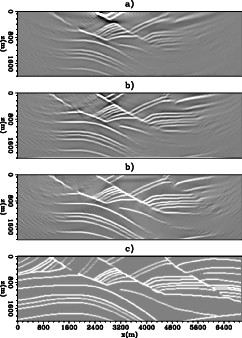
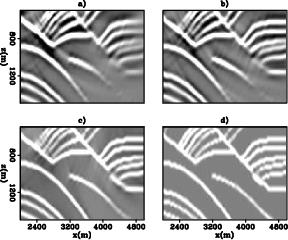
Panels (a) and (b) of Figure 6 show the corresponding up-image and down-image. Comparing the two images, we can see that wider illumination is achieved by the mirror image. The benefit of the wider aperture is directly correlated with the depth of the sea-bottom. The deeper the sea-bottom, the wider the illumination. On the other hand, a close-up section of the images (Figure 7 (a) and (b)) shows that the up-image has a higher signal-to-noise ratio than the down-image. This is only a synthetic study and we expect the difference will be more apparent with a field dataset.

RTM
Figure 6. (a) Up-image obtained by calculating $\mathbf L_{\uparrow}^{'} \mathbf d_{\uparrow}^{mod}$ , (b) down-image obtained by calculating $\mathbf L_{\downarrow}^{'} \mathbf d_{\downarrow}^{mod}$ , (c) image obtained by joint inversion, and (d) reflectivity model.

DIcom
Figure 7. A section of the image cut from x=2500-4500 m and y=500-1500 m. Images are clipped at 90% to contrast the quality among (a) the up-image, (b) the down-image, (c) the joint-image, and (d) the model.

The goal of joint inversion is to get the best of both worlds. By manipulating two sets of data, we wish to produce a joint image that has both the wide illumination of the down-image and a high signal-to-noise ratio in the region covered by the up-image.

Joint least-squares inversion of up- and down-going signal for ocean bottom data sets