Predicting rugged water-bottom multiples through wavefield extrapolation with rejection and injection

Synthetic example

To evaluate the usefulness of multiple prediction and adaptive subtraction, we use the geologic model shown in figure 4 to produce the synthetic seismic data. In this model, there are four layers, including the water layer. The interval velocities from the top to bottom layer are 1500, 2500, 3500 and 4500 m/s respectively, and the depths of the first to third interface are 1000, 2000 and 3000 m respectively. As there is a notch (trench) on the first interface, the synthetic seismic data contain not only specularly reflected but also diffracted water-bottom multiples and peg-legs. Furthermore, the model has a convex feature (fault or salt) on the third interface to produce specularly reflected and diffracted interbed multiples. In addition, to test the ability to preserve the primary, we design the interface depths such that the zero-offset travel time of the first order water-bottom multiples are very close to the zero-offset reflection time of the third interface. Figure 5 and figure 6 show shot gathers and predicted multiples at the leftmost and central locations. Figure 7 shows the zero-offset sections of the original seismic data and predicted multiples. Comparing the original and predicted multiples both in the shot gathers and the zero-offset section, we can see that both the specularly reflected and diffracted water bottom multiples and peg-legs are well predicted. The results also demonstrate the limitation of both the convolution-based and WEM-modeling-based surface-related multiple prediction methods; neither can predict the interbed multiples.

smcof1
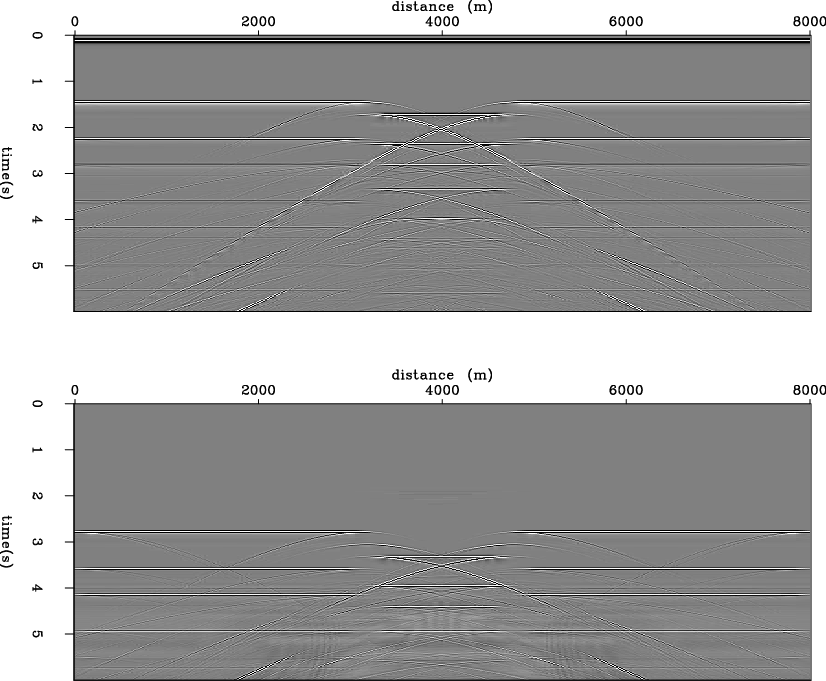
Figure 7. The zero-offset sections of the original seismic data (top) and the predicted multiples (bottom). [NR]

Predicting rugged water-bottom multiples through wavefield extrapolation with rejection and injection