Applications of the generalized norm solver

Result of least-squares inversion of the 1D Galilee Problem

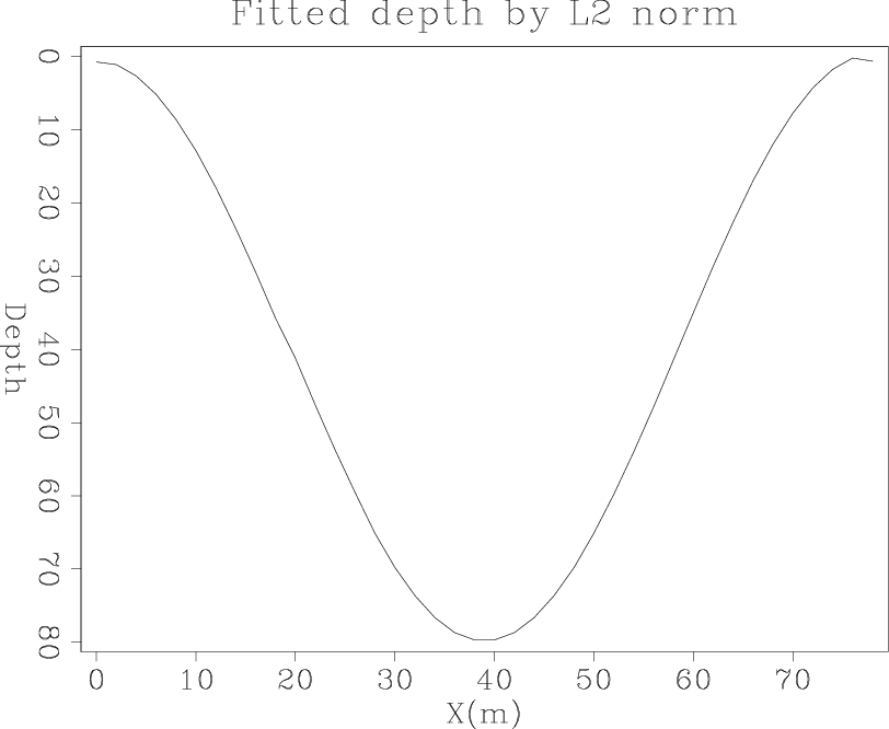
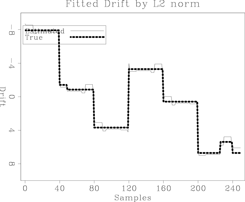
Least-squares inversion looks a for solution in the model space that minimizes the square of the residual. I first run un-regularized inversion on spike-free but drifted data. That means using the data-fitting goal in equation 3 to fit the data shown from Figure 3 (b). After L2 fitting, the estimated depth is shown in figure 4 (a), and the estimated drift is shown in figure 4 (b). An interesting observation from the un-regularized L2 inversion of the non-spike data is that it gives very good estimate of the lake depth and drift. Although the problem is still under-determined, the amount of data collected is sufficient enough to determine the relative jumps from each pass in the lake. As mentioned before, the data cover the lake back and forth roughly 6.25 times.

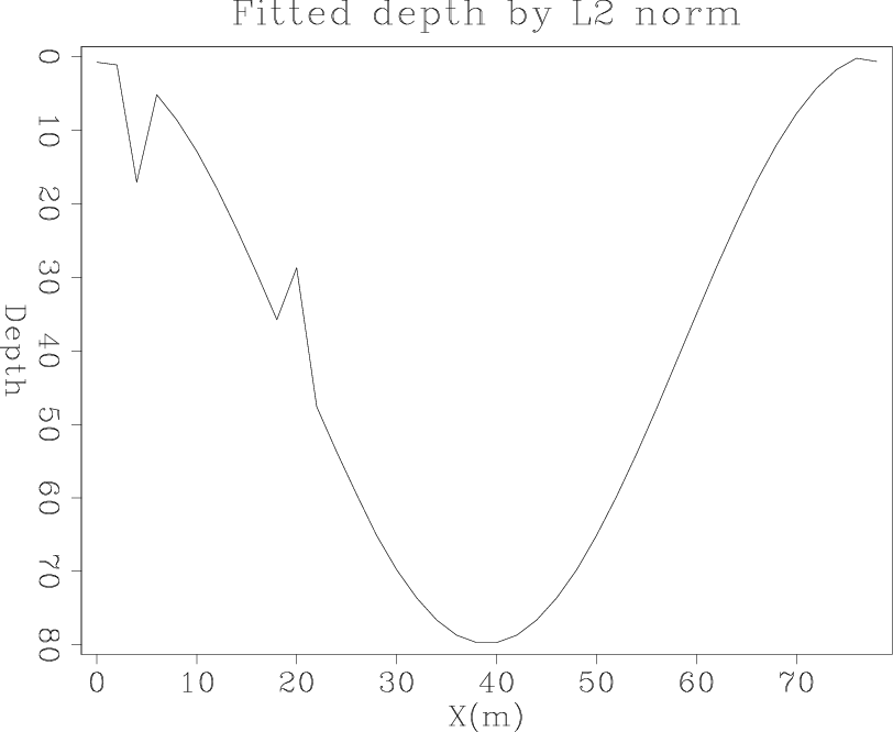
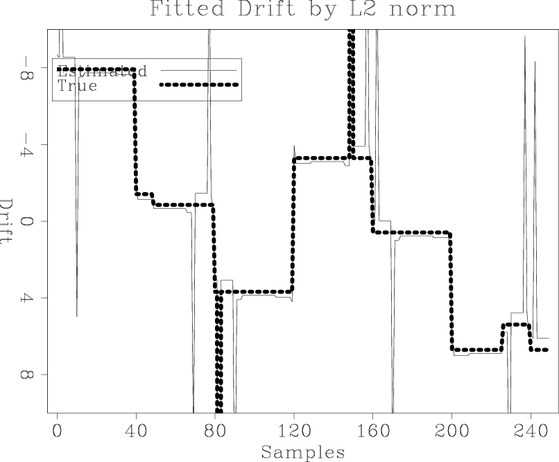
At this point, further attempts to solve this problem seem redundant, as we are getting a nearly perfect result. However, the result is different when I re-run the un-regularized inversion (equation 3) on the spiked and drifted data (Figure 3 (c)). After L2 fitting, the estimated depth is shown in figure 4 (c),and while the estimated drift is shown in Figure 4 (d). This time, the fitted depth deviates from the true depth, with segments that are clearly affected by spikes. The fitted drift function shows erratic jumps. This is because by minimizing the square of the residual, L2 inversion emphasizes large spikes in data. In a situation like this, L1 or L1-type inversion like the hybrid and Huber solvers should give better results. This is because minimizing the absolute value of the residual puts less emphasis on large spikes in data. This assertion will be verified when I apply the hybrid and the Huber solvers in the next section.

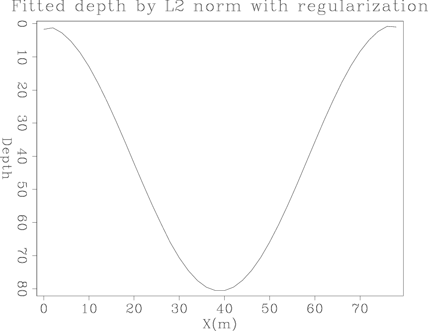
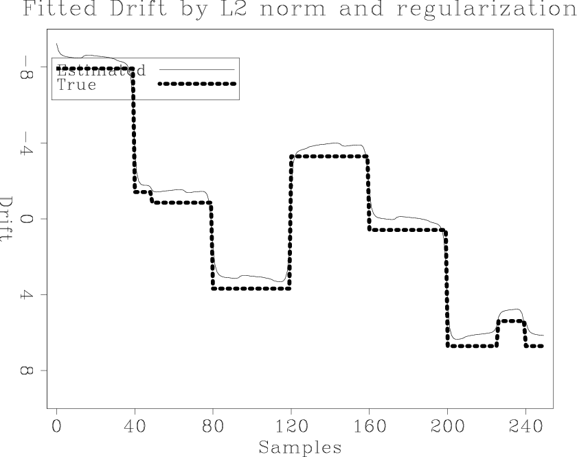
In addition to the two un-regularized least-squares examples above, I also ran a regularized inversion on the spike-free but drifted data. That means using the fitting goals in equation 3 and equation 4 on the data shown in Figure 3 (b). After L2 fitting, the estimated depth is shown in Figure 4 (e), and the estimated drift is shown in Figure 4 (f). The regularized drift in this case, shown in Figure 4 (f) , is a smoothed version of the un-regularized drift as shown in Figure 4 (b). The smoothing is as expected because of the type of regularization used. One conclusion is that when the data is spike-free, the L1-type solver is unnecessary, because Figure 4 (b) shows that we are obtaining a satisfactory result with L2 unregularized fitting. However, Figure 4 (d) demonstrates that L1-type inversion is needed for data containing large spikes. The next step is to see how the generalized L1 solver handle this problem using the hybrid and the Huber norms.

l2dpt1,l2drf1,l2dpt0,l2drf0,l2dpt2,l2drf2
Figure 4. (a,b): L2 inversion without regularizaton using the spike-free data. (c,d): L2 inversion without regularization using the spiked data. (e,f): L2 inversion with regularization using the spike-free data. [ER]

Applications of the generalized norm solver