Dix inversion constrained by L1-norm optimization

Synthetic and field data example

Figure 1 shows the input synthetic RMS velocities with and without random noise, and the true blocky interval velocity we try to invert for. For the synthetic problem, we experimented on solvers with and without regularization to learn the nature of the solver itself and the nature of its regularization.

Figure 2 shows the inversion results when clean data (free of noise) are fed into different simple solvers without any regularization. The result of $L2$ regression is comparable to the IRLS and hybrid norm. However, the simple conjugate direction $L1$ solver failed to give a satisfactory result (Figure 2(c)). As we have discussed in the previous section, this might be due to the flat bottom caused by the data configuration.

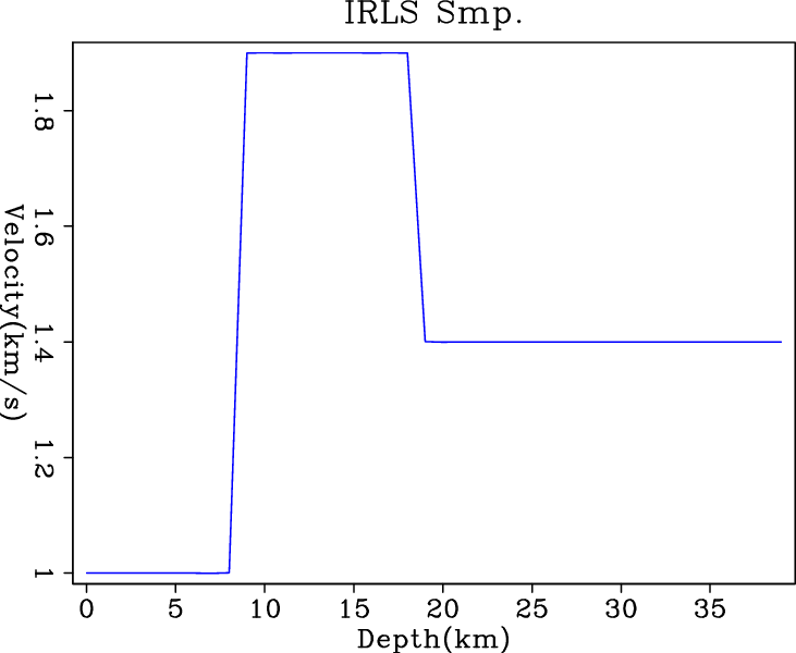
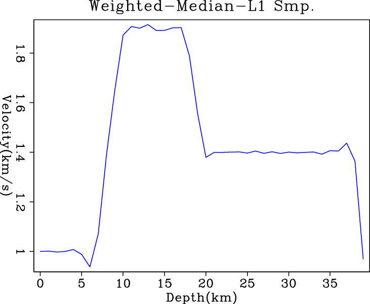
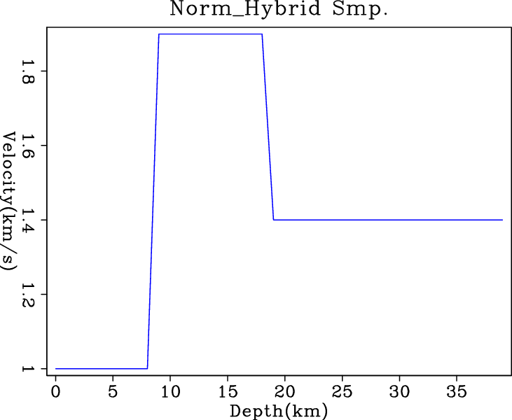
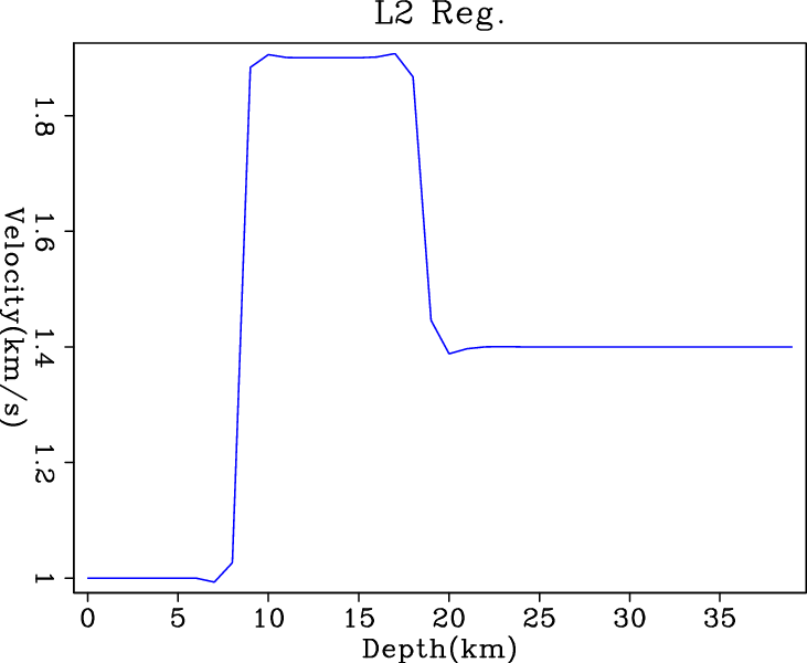
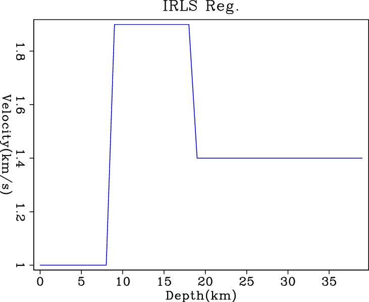
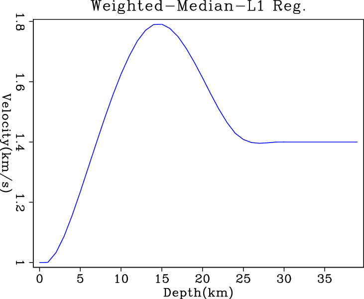
Figure 3 shows the inversion results when clean data are fed into different regularized solvers. As expected, the smoothing effect of $L2$ regularization on the derivative of model produces the round corners at the turning point. In contrast, IRLS and hybrid solvers give perfect exact solutions, which benefit from their $L1$ nature in regularization. We do not fully understand the behavior of conjugate-direction $L1$ solver, but the change in the result can be explained by the change of the data configuration when the regularization term is added.

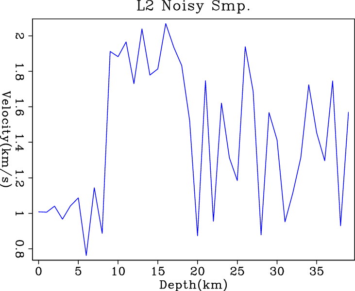
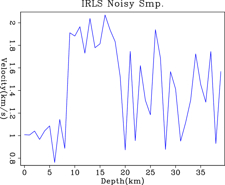
Figure 4 shows the inversion results when noisy data are fed into different simple solvers without any regularization. When creating the synthetic noisy RMS velocity data, uniform distributed random noise is added. However, $L2$ norm assumes Gaussian noise, and $L1$ minimization is derived under the assumption of exponential distribution. Therefore, the simple $L2$ solver, the IRLS solver or hybrid solver all fail to recognize the noise and attenuate it. Surprisingly, conjugate-direction $L1$ solver successfully eliminates the high-frequency noise and keeps the low-frequency trend of the interval velocity function. It shows great potential for finding the exact solution when the problem is slightly more complicated.

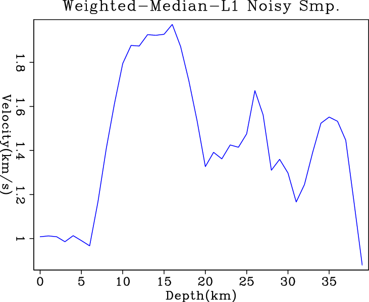
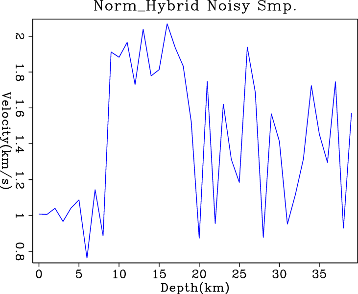
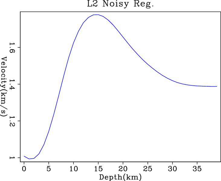
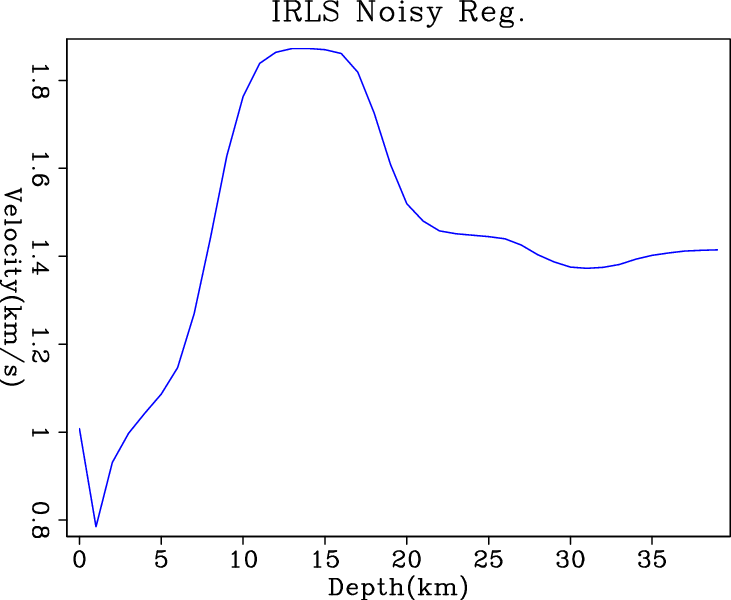
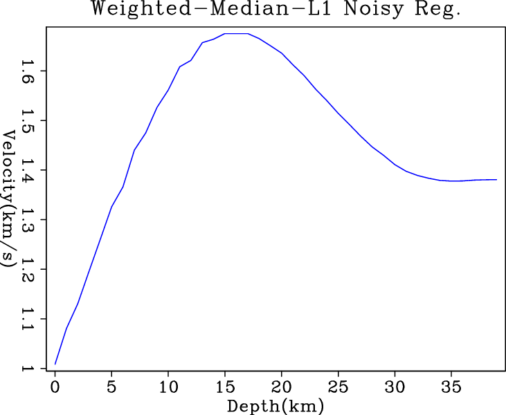
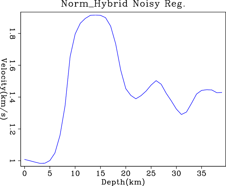
Figure 5 shows the inversion results when noisy data are fed into different regularized solvers. By adding this regularization term to further constrain the problem, we expect better results out of each solver. Comparing the results in Figure 5, IRLS result has the most blocky transition between layers and is almost flat within the layers. However, the big jump at shallower depths is apparently due to its tolerance of the large residuals. The hybrid solver gives result comparable to the IRLS, but it oscillates at deeper depths. The results from $L2$ and conjugate direction $L1$ solver are similar, but the smaller steps in the result of conjugate direction $L1$ (Figure 5(c)) are promising.

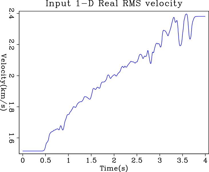
Figure 6 shows the 1-D field RMS velocity from the velocity scan. This field data has 1,000 sample points, and the number of blocks in the model space is unknown. In real life, we can never fully constrain a inversion problem without regularization: that is when Dix inversion becomes unstable. Therefore, only regularized solvers are tested.

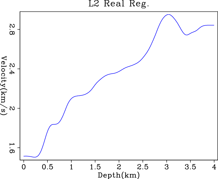
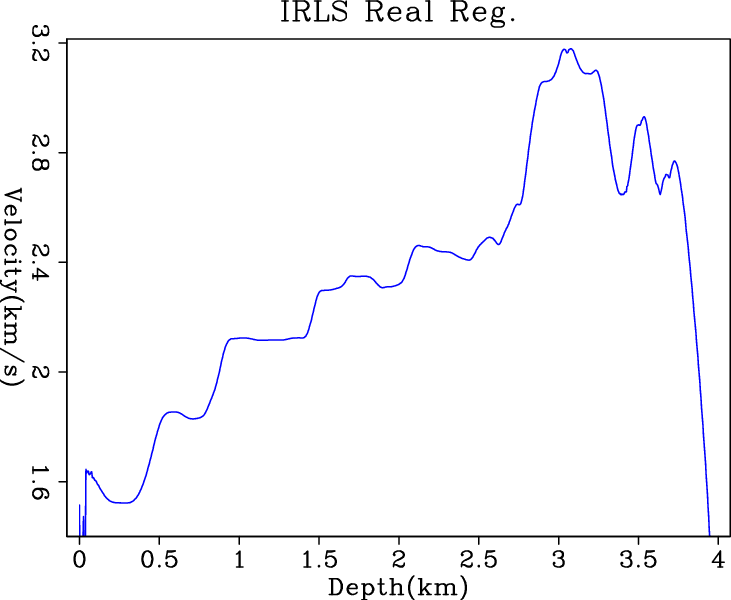
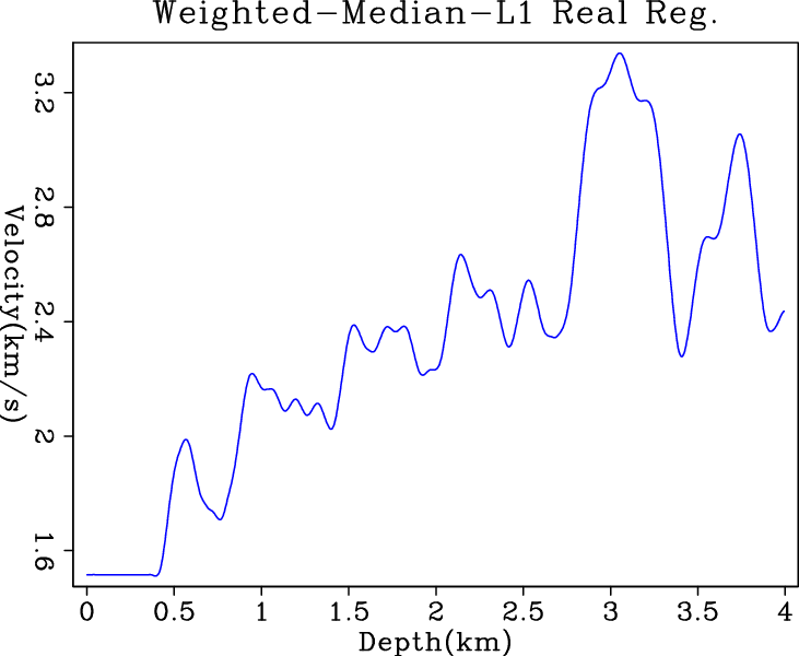
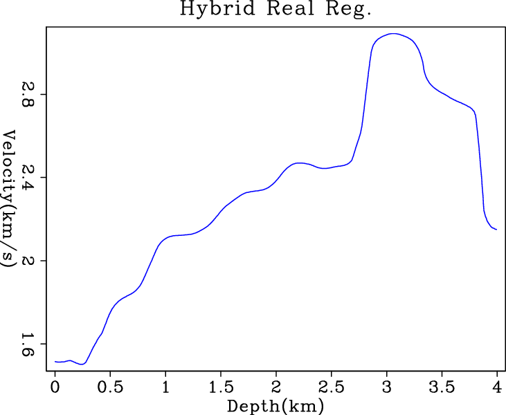
Figure 7 shows the inversion results when field data in Figure 6 are fed into different regularized solvers. The results from the IRLS and the conjugate direction $L1$ solver have more blocky nature than the other two. The result from IRLS is more flat within layers, which is a nice property in well-log matching and many other geophysical applications. The hybrid and $L2$ solvers give comparable results, although we have chosen a very small $\sigma$ for hybrid norm to force it towards the $L1$ norm.

rmsvel,rms-noise,intervel
Figure 1. Input synthetic RMS velocity and true interval velocity. The two plots on the top row are the input RMS velocities (a) without noise and (b) with random noise, respectively. The plot on the bottom is (c) the true interval velocity which is true model in the estimation problem. [ER]

l21,irls1,wmed1,nrm3
Figure 2. Inversion results of simple (a) $L2$ solver; (b) IRLS solver; (c) conjugate direction $L1$ solver and (d) Hybrid solver when clean data are fed in. All the regressions are without regularization. [ER]

l22,irls2,wmed2,nrm2
Figure 3. Inversion results of (a) $L2$ solver; (b) IRLS solver; (c) conjugate direction $L1$ solver and (d) Hybrid solver when clean data are fed in. All the regressions are regularized.[ER]

l23,irls3,wmed4,nrm5
Figure 4. Inversion results of simple (a) $L2$ solver; (b) IRLS solver; (c) conjugate direction $L1$ solver and (d) Hybrid solver when noisy data are fed in. All the regressions are without regularization.[ER]

l24,irls4,wmed5,nrm6
Figure 5. Inversion results of (a) $L2$ solver; (b) IRLS solver; (c) conjugate direction $L1$ solver and (d) Hybrid solver when noisy data are fed in. All the regressions are regularized. [ER]

realrms Figure 6. Input 1-D field RMS velocity data from velocity scan. [ER]

real2,real1,real4,real6
Figure 7. Inversion results of (a) $L2$ solver; (b) IRLS solver; (c) conjugate direction $L1$ solver and (d) Hybrid solver when 1-D field RMS velocity data are fed in. All the regressions are regularized. [ER]

Dix inversion constrained by L1-norm optimization