Selecting the right hardware for Reverse Time Migration

Domain decomposition and resampling

Domain decomposition involves splitting our computation domain into several sub-domains. Figure 2 shows how each sub-domain is then marched forward in time (one or more steps) separately. Domain decomposition can be done at the core, processor, or node level. Different computational units are assigned different portions of the domain. They are responsible for computing an updated solution in their region.

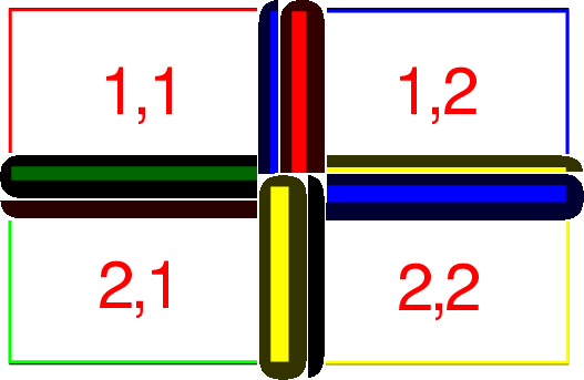
decomposition Figure 2. An example domain decomposition. The domain is broken into four portions reducing the amount of memory needed and/or reducing cache misses improving performance. The domains can not be treated completely indepently because the rely on retrieving information from the neighbors as the time marching scheme progresses.[NR]

The primary advantage of this approach is that each sub-domain is smaller, increasing the likelihood that the cache line will be close (in L1 or L2 cache) rather flushed to main memory. A more subtle advantage of domain decomposition is that sub-domains can represent significantly different velocity ranges, and therefore different spatial sampling requirements to obtain the same level of accuracy, stability, and dispersion. These modifications can potentially allow significant performance gains.

Naturally, there are also disadvantages. First, notice the shaded squares in Figure 2 that demonstrate that a sub-domain must access some of its neighbors' elements in order to calculate the spatial derivative along its own edge. As a result, there is a limit on how independently each sub-domain can operate and how small the sub-domains can become before the cost of rereading or passing the boundary region becomes the dominant cost. In addition, transferring this boundary region from one computational unit to another can become a bottleneck. Calculating derivatives at the boundaries and potentially handling load balancing can make the code considerably more complex.

Selecting the right hardware for Reverse Time Migration