 |
 |
 |
 | Theory and practice of interpolation in the pyramid domain |  |
![[pdf]](icons/pdf.png) |
Next: Examples
Up: Algorithm for missing data
Previous: Mitigating mapping effects
We are now ready to present the missing data interpolation algorithm. One
side effect of the fine sampling of the  axis is that empty bins
will appear in the pyramid domain. Missing data in
axis is that empty bins
will appear in the pyramid domain. Missing data in  will add
even more empty locations. We propose interpolating the missing data
in by filling the empty bins in
will add
even more empty locations. We propose interpolating the missing data
in by filling the empty bins in 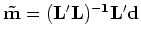 . For this, we follow
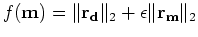
the approach of Claerbout and Fomel (2002). First, we want to honor the data where
they are known by introducing the residual vector
. For this, we follow
the approach of Claerbout and Fomel (2002). First, we want to honor the data where
they are known by introducing the residual vector
 |
(13) |
where  is a masking operator equal to unity where data
are known, and zero where data are missing. Solving for
minimizing the amplitude of
is a masking operator equal to unity where data
are known, and zero where data are missing. Solving for
minimizing the amplitude of  only will not fill the empty
bins. We need to add a regularization term
that will enforce a certain multivariate spectrum to the vector :
only will not fill the empty
bins. We need to add a regularization term
that will enforce a certain multivariate spectrum to the vector :
 |
(14) |
where  is a pef in the model space. Assuming that the pef
is known, we can fill the empty locations in by
minimizing
is a pef in the model space. Assuming that the pef
is known, we can fill the empty locations in by
minimizing
 , where
 is a balancing operator between data fitting and model space
regularization.
is a balancing operator between data fitting and model space
regularization.
There are two issues with this approach.
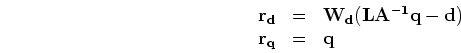
The first issue is that the convergence towards a solution will be slow. To accelerate
this process we introduce a new variable
 and rewrite equations
(13) and (14) as follows:
and rewrite equations
(13) and (14) as follows:
 |
(15) |
We then minimize
 and compute
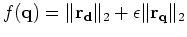 , where
  minimizes
  .
The term
.
The term  is computed by applying a polynomial division
to
is computed by applying a polynomial division
to  which yields fast filling of the empty bins. Because is a
miminum-phase filter, the polynomial division is stable and will not cause the solution
to blow-up.
This preconditioning of the problem has been used in numerous geophysical problems
[Herrmann et al. (2009); Fomel and Guitton (2006); Clapp et al. (2004)]. In practice, we set
which yields fast filling of the empty bins. Because is a
miminum-phase filter, the polynomial division is stable and will not cause the solution
to blow-up.
This preconditioning of the problem has been used in numerous geophysical problems
[Herrmann et al. (2009); Fomel and Guitton (2006); Clapp et al. (2004)]. In practice, we set
 and minimize only [Trad et al. (2003); Guitton and Claerbout (2004)].
The second issue is that both and are unknown in
equation (15). To circumvent this problem we bootstrap
the pef estimation by first assuming that is a 1-D gradient.
To make sure that we can apply the polynomial division, we set the second coefficient of the
gradient to  instead of
  . We then minimize
with this first pef, find a new
. We then minimize
with this first pef, find a new  and estimate a better
pef from it. Having a better pef, we can minimize again:
and estimate a better
pef from it. Having a better pef, we can minimize again:

iterate {
minimize  )
)

estimate from
}
We are essentially solving the non-linear problem in a
step-wise fashion by keeping constant within each non-linear
loop. In practice, we notice that only 4 to 5 non-linear iterations
are necessary to converge towards a pef that yields accurate
interpolation of the missing data.
In the next section, we apply this algorithm to synthetic and field
data examples in 2-D. We show that aliased and irregularly-sampled data can be
interpolated.
|
|
|
|
| Theory and practice of interpolation in the pyramid domain | |
|
Next: Examples
Up: Algorithm for missing data
Previous: Mitigating mapping effects
2009-10-19