Seismic tomography with co-located soft data

Application of the cross-gradient function in seismic tomography

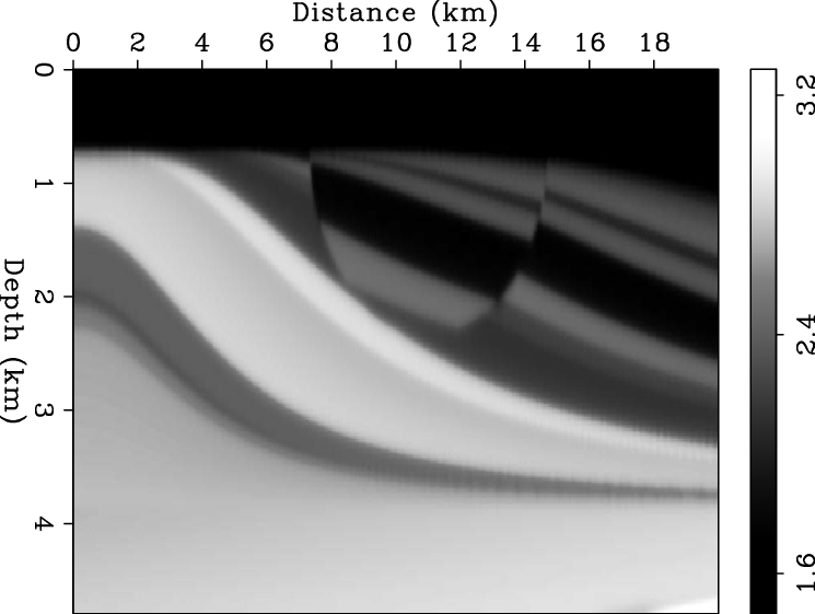
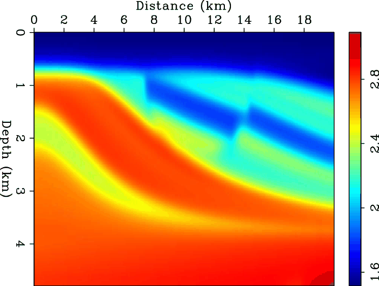
Figure 3 shows a velocity map and corresponding resistivity map of a synthetic 2-D model. That includes a water velocity of about $1.5 \frac{km}{s}$ at the top and a semi-circular fault in the middle of the ocean bottom. There are also laterally smooth velocity anomalies in the model. The resistivity profile and velocity profile are connected using the Archie/time-average cross-property relation (Carcione et al., 2007) with arbitrary parameter values.

vel-t,softdata1-0
Figure 3. Synthetic sinusoidal model with (a) two velocity anomalies and corresponding (b) resistivity model. [ER]

We use the resistivity map as soft data to constrain the tomography problem with the cross-gradient function. In this case, we can write the cross-gradient function given in equation 2 as a linear operator $\mathbf{G}$ on the slowness field, $\mathbf{s}_0+\Delta \mathbf{s}$. We can then extend the linearized tomography problem by employing $\mathbf{G}$ as an additional constraint. The objective function, $\mathcal{P} (\Delta \mathbf{s})$, of this extended problem becomes

$$\mathcal{P} (\Delta \mathbf{s}) =\vert\vert\Delta \mathbf{t} - \m... ...psilon_1^2 \vert\vert \mathbf{G} (\mathbf{s}_0+\Delta \mathbf{s})\vert\vert^2,$$ (6)

where $\epsilon_1$ is a problem-specific weight factor to regularize the tomography problem (Clapp, 2001).

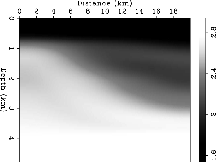
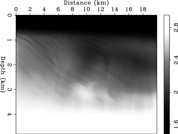
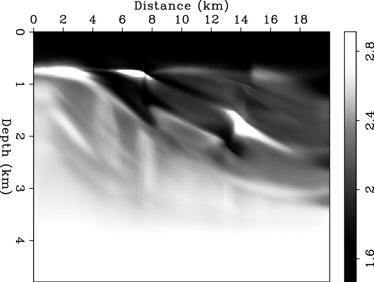
Figure 4 shows the initial velocity and the estimated velocities found by solving the tomography problem both with steering filters and the cross-gradient constraint.

vel-0,vel-ds0,velx-dsx0
Figure 4. Velocity estimates by seismic tomography: Initial velocity estimate (a) and estimated velocity (b) with steering filers and (c) with cross-gradient constraint on soft-data. [CR]

The results show that steering filters yield a good result for low frequency features such as smooth lateral velocity anomalies; however, it ignores high-frequency structures of the velocity model. On the other hand, the cross-gradient functions are able to provide better estimates for high-frequency features of the velocity model, such as sharp salt boundaries and faults. Steering filters assume a priori knowledge of the model parameters, while the cross-gradient function uses the co-located soft data field to build this information. The combination of these two method may be an optimal tool for addressing the velocity estimation problem in more general subsurface structures.

Seismic tomography with co-located soft data