Delayed-shot migration in TEC coordinates

Narrow-azimuth field data test

This section presents the results of applying the inline delayed-shot imaging procedure to a 3D Gulf of Mexico narrow-azimuth data set provided by ExxonMobil. The velocity model, shown in Figure 11, consists of typical sediment-controlled $v(\xi_3)$ velocity structure, save for the salt body intruding in the center of the block, and offset associated with throw along the moderately dipping fault planes. By agreement with ExxonMobil, the depths shown in all figures differ from the true values.

XOM-VEL
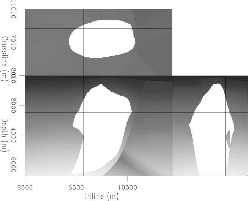
Figure 11. Velocity model example for Gulf of Mexico field data set. ER

Key imaging targets in this model include the steep salt flanks around the salt structure and the onlapping sediments. Previous imaging work in this area indicates that the sediments surrounding the salt body exhibit moderate-to-strong degrees of anisotropy. Bear et al. (2005) estimated the vertical velocity and anisotropy parameters (assuming VTI media) using a joint inversion technique that combined surface seismic and borehole constraints. Shan (2008), using a 3D tilted Cartesian coordinate plane-wave migration algorithm for transversely isotropic (TTI) media, demonstrated that accounting for anisotropy greatly improves migrated image quality for this data set.

The migration strategy presented herein differs from that in Shan (2008) in a number of respects. First, I perform migration using only isotropic vertical-velocity sediment flood model that does not incorporate anisotropy. Second, I use a multi-streamer data set for imaging, rather than the more optimally regularized single-streamer data formed through azimuthal move-out preprocessing (Biondi, 2004).

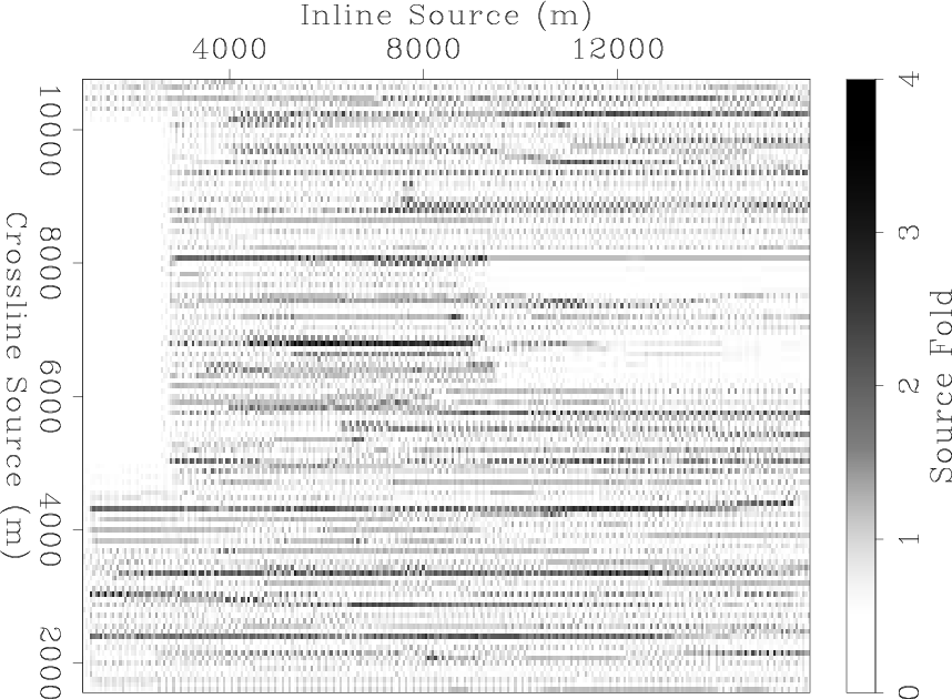
Table 4 summarizes the acquisition geometry of the data set. The data used for migration consisted of 54 sail lines separated roughly 160 m apart, each sail line consists of approximately 300 shots acquired every 50 m.

Table 4: Approximate acquisition parameters associated with the 3D Gulf of Mexico field data set.

Source Parameter	Value	Receiver Parameter	Value
Number of sail lines	54	Max. inline offset (m)	$\pm$3725
Sail line interval (m)	160	Max. crossline offset (m)	$\pm$500
Shots per sail line	300	Inline receiver interval (m)	25
Shot interval (m)	50	Crossline receiver interval (m)	80

I binned the sources in 25 m and 80 m intervals in the inline and crossline, respectively. Figure 12 shows the source distribution, and illustrates the sail line direction, herein chosen to be the inline direction. Figure 13 shows the chosen offset distribution. The receiver points fall to both positive and negative offsets, as the sail lines were acquired in two directions. The gap in offset coverage between offsets of $\pm$2500-2750 m arises due to a corrupted data tape. Receivers were binned at 25 m in both the inline and crossline directions.

XOM-SRC Figure 12. Chosen source distribution for the field data set. CR

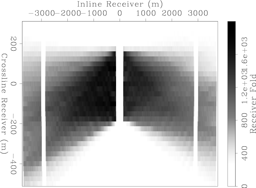
XOM-RCV Figure 13. Chosen receiver distribution for the field data set. The missing data between offsets $\pm$2500-2750 m is due to a corrupted data tape. CR

I prepared the data for migration by applying an inline delay-shot phase-encoding algorithm according to the inline source position. A total of 54 plane-wave sub-volumes were generated from the total 5D shot record volume, each consisting of 41 plane-waves equally sampled between $\pm 20^\circ$. I chose a total of 244 frequencies between 3 Hz and 25 Hz for migration. The data were imaged on migration grids with dimensions of 800x350x300 samples. Migrations in TEC coordinates were performed using tilt angles between $\pm 20^\circ$ at $1^\circ$ increments.

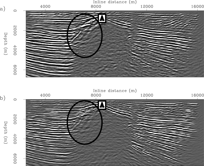
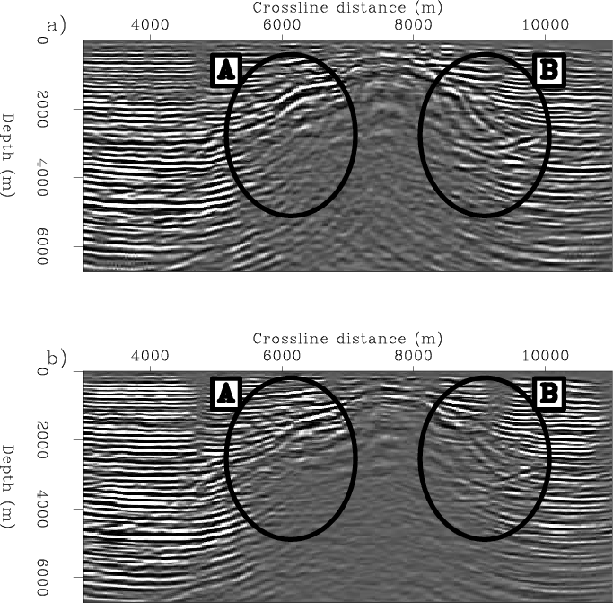
Figures 14-16 present comparative slices from the 3D Gulf of Mexico migration images computed in the TEC and Cartesian coordinate systems. Figure 14 presents an inline section taken at the constant 8750 m crossline coordinate for the TEC (top panel) and CC (bottom panel) images corresponding to the front face of Figure 11. The top of salt body is well-imaged in both images; however, the near-vertical salt-flanks to the right are nearly entirely absent. Oval A shows the imaging improvements in TEC coordinates for the left-hand flank.

RFIG1
Figure 14. Inline sections through the migration images taken at the 8750 m crossline coordinate location. Top: TEC coordinate migration results. Bottom: Cartesian coordinate migration results. Oval A shows the imaging improvements in TEC coordinates for the left-hand flank. CR

Figure 15 presents crossline sections for the TEC (top panel) and CC (bottom panel) images. Both images are subject to fair amounts of near-surface aliasing a sali line contribution every 160 m in the crossline direction, as well as the artifaces due to using a non-regularized data set with locations where no data are present. The outlines of the salt body reflector, though, are imaged. Oval A shots an example of an area where the TEC coordinate image is better than the Cartesian image.

RFIG3
Figure 15. Crossline sections through the migration images taken at the 7100 m crossline coordinate location. Top: TEC coordinate migration results. Bottom: Cartesian coordinate migration results. Oval A shows an example of an area where the TEC coordinate image is better than the Cartesian image. CR

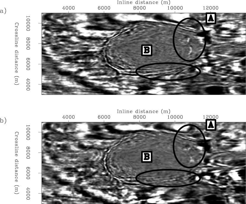
Figure 16 presents a depth slice extracted from the TEC (top panel) and CC (bottom panel) image volumes. The annular ring, showing the location of the salt body, is apparent in both images; however, the image is sharper in the TEC image indicating improved focussing of energy. Oval A shows an example of an area where the TEC image is better than that generated in Cartesian, including two parts of the right-hand salt flank. Oval B shows the TEC coordinate image improvements in the crossline direction.

RFIG5
Figure 16. Migration results for the 3D Gulf of Mexico field data set through the sedimentary section. Top: TEC coordinate migration results. Bottom: Cartesian coordinate migration results. Oval A shows an example of an area where the TEC image is better than that generated in Cartesian, including two parts of the right-hand salt flank. Oval B shows the TEC coordinate image improvements in the crossline direction. CR

The results of the 3D field data application likely could have been improved in a number of aspects. First, a migration velocity model incorporating anisotropy values (e.g. $v_{mig} = v_{vert}(1+1.8\delta)$) could have been used instead of the vertical velocity profile. Although this would affect the vertical location of the flat-lying sedimentary reflectors, it likely would have led to more accurate horizontal propagation and imaging of waves reflecting off the target salt flanks. Second, if additional computational resources were made available, migrating the full data set (i.e. every 80 m in crossline source position rather than every 160 m) with a higher frequency content would have led to a more infilled and higher resolution image. Third, extending the generalized RWE theory to incorporate TTI anisotropy likely would have enabled a more consistent imaging of the steep salt flanks. This extension is likely to be a subject for future research.

Delayed-shot migration in TEC coordinates