 |
 |
 |
 | Target-oriented joint inversion of incomplete time-lapse seismic data sets |  |
![[pdf]](icons/pdf.png) |
Next: About this document ...
Up: Linear least-squares modeling/inversion
Previous: Linear least-squares modeling/inversion
The large computational cost of full Hessian (equation A-4) makes explicit computation impractical.
Previous authors (Symes, 2008; Guitton, 2004; Shin et al., 2001; Rickett, 2003; Valenciano, 2008; Plessix and Mulder, 2004) have discussed possible approximations that reduce the computational cost or remove the need for explicit computation of the full Hessian.
Because reservoirs are limited in extent, the region of interest is usually smaller than the full image space, therefore, the Hessian can be explicitly computed for that region.
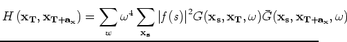
For our problem, we follow the target-oriented approximation (Valenciano, 2008) to the Hessian, which for a target region
 is
is
 |
|
|
|
 |
|
|
(A-5) |
where
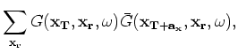 represents a small region around each point within
.
For any image point,
represents a small region around each point within
.
For any image point,
 represents a row of a sparse Hessian matrix
  whose non-zero components are defined by
 .
The term,
, which can be estimated as a function of the decrease in amplitude of the Hessian diagonal, defines the filter-size around each image point.
Valenciano (2008) discusses the target-oriented Hessian in detail and reviews the computational savings from this approximation.
.
The term,
, which can be estimated as a function of the decrease in amplitude of the Hessian diagonal, defines the filter-size around each image point.
Valenciano (2008) discusses the target-oriented Hessian in detail and reviews the computational savings from this approximation.
|
|
|
|
| Target-oriented joint inversion of incomplete time-lapse seismic data sets | |
|
Next: About this document ...
Up: Linear least-squares modeling/inversion
Previous: Linear least-squares modeling/inversion
2009-05-05