|
|
|
|
Automatic velocity picking by simulated annealing |
The simulated annealing (SA) algorithm is the computational analog of slowly cooling a metal so that it adopts a low-energy, crystalline state. It is a provably convergent optimizer. Geman and Geman (1984) provided a proof that simulated annealing, if the annealing is sufficiently slow, converges to the global optimum. In geophysics, SA has been employed to solve the problems of statics (Rothman, 1985), waveform inversion (Sen and Stoffa, 1991) and ray tracing (Bona et al., 2009). Here we propose the application of the simulated annealing algorithm to automatic velocity picking.
We initialize the system at a high temperature. At this stage the particles are then free to move around by a small pertubation; as the temperature is lowered, however, they are increasingly confined due to the high energy cost of movement. At each temperature T, SA perturbs the system randomly until it reaches equilibrium. The new state of the perturbed system is accepted according to the metropolis algorithm:
| (1) |
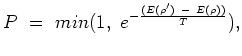 is the perturbed
velocity model, and E is the objective function presented later in the
chapter. As shown in the equation, a higher T introduces a
higher probability that an uphill perturbation will be accepted,
which means that SA can draw samples from the whole population. As T
decreases, only perturbations leading to smaller increases in E
are accepted, so that only limited exploration is possible as the
system settles to the global minimum. The pseudo code of the
algorithm is given in Table 1.
is the perturbed
velocity model, and E is the objective function presented later in the
chapter. As shown in the equation, a higher T introduces a
higher probability that an uphill perturbation will be accepted,
which means that SA can draw samples from the whole population. As T
decreases, only perturbations leading to smaller increases in E
are accepted, so that only limited exploration is possible as the
system settles to the global minimum. The pseudo code of the
algorithm is given in Table 1.
The simulated annealing algorithm is popular and has been
well-developed for single-objective optimization. Traditionally,
multiobjective optimization can be converted into a single-objective
optimization by different fix-up approaches such as the weighted-sum
or ![]() -constraint method. In our case, we use a
composite-objective function:
-constraint method. In our case, we use a
composite-objective function:
| (2) |
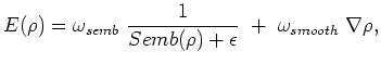 is the inverse of semblance and is a
measurement of focusing;
is the inverse of semblance and is a
measurement of focusing; There are different ways to compose this single objective function. By using the inverse of semblance and residual of Laplacian we cast the optimization as a minimization problem. This combined objective function is then used as the energy or cost to be minimized in an SA optimizer. For the case we discuss here, the fixed weights are chosen according to the relative importance of the objective functions.
|
|
|
|
Automatic velocity picking by simulated annealing |