|
|
|
|
Modeling, migration, and inversion in the generalized source and receiver domain |
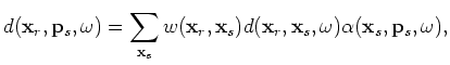 )and
receivers (
)and
receivers (
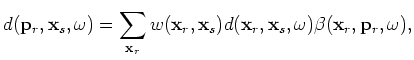 ) need not be the same.
For example, we can use plane-wave phase encoding function to encode the sources but use random phase-encoding function
to encode the receivers, or vice visa. Because plane-wave phase encoding functions are very effective in attenuating the cross-talk (Tang, 2008; Liu et al., 2006),
while random phase encoding is efficient, by combining those two phase-encoding functions, we are able to balance cost and accuracy.
) need not be the same.
For example, we can use plane-wave phase encoding function to encode the sources but use random phase-encoding function
to encode the receivers, or vice visa. Because plane-wave phase encoding functions are very effective in attenuating the cross-talk (Tang, 2008; Liu et al., 2006),
while random phase encoding is efficient, by combining those two phase-encoding functions, we are able to balance cost and accuracy.
I apply this idea to a simple constant-velocity model. The acquisition geometry is assumed to be OBC geometry, where all shots share the same receiver array.
There are ![]() shots from
shots from ![]() m to
m to ![]() m with a
m with a ![]() m sampling; for each shot, there are
m sampling; for each shot, there are ![]() receivers spanning from
receivers spanning from ![]() m to
m to ![]() m.
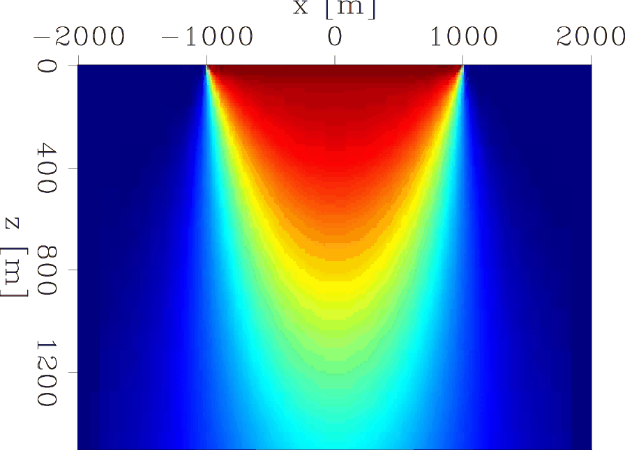
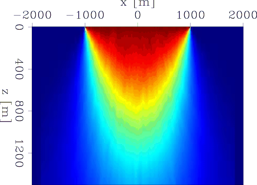
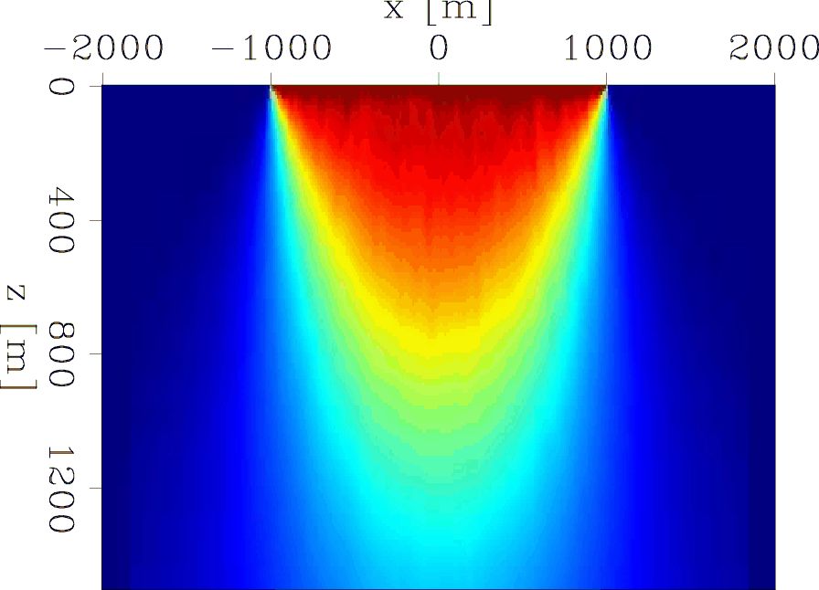
Figure 2 shows the diagonal of the Hessian obtained using different methods.
Figure 2(a) shows the exact diagonal of the Hessian computed in the original shot-profile domain with Equation 7,
which requires pre-computing and saving the Green's functions and is efficient for practical applications.
However, since there is no cross-talk in the original shot-profile domain, I use the result as a benchmark to compare the accuracy of other methods.
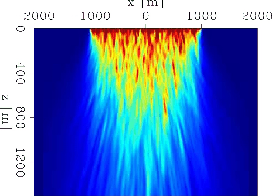
Figure 2(b) is obtained using the most efficient simultaneous random phase-encoding method
(only one realization of the random-phase functions has been used),
by using Equation 33, with both
and
being
random phase functions. As expected, the result is full of random noise, useful illumination information is greatly distorted, and the result is very
far from the exact Hessian. Figure 2(c) shows the result obtained using the mixed phase-encoding scheme,
i.e., by using Equation 33, with the weighting function
being the
plane-wave phase-encoding function and
being the random phase-encoding function.
A total of
m.
Figure 2 shows the diagonal of the Hessian obtained using different methods.
Figure 2(a) shows the exact diagonal of the Hessian computed in the original shot-profile domain with Equation 7,
which requires pre-computing and saving the Green's functions and is efficient for practical applications.
However, since there is no cross-talk in the original shot-profile domain, I use the result as a benchmark to compare the accuracy of other methods.
Figure 2(b) is obtained using the most efficient simultaneous random phase-encoding method
(only one realization of the random-phase functions has been used),
by using Equation 33, with both
and
being
random phase functions. As expected, the result is full of random noise, useful illumination information is greatly distorted, and the result is very
far from the exact Hessian. Figure 2(c) shows the result obtained using the mixed phase-encoding scheme,
i.e., by using Equation 33, with the weighting function
being the
plane-wave phase-encoding function and
being the random phase-encoding function.
A total of ![]() plane-wave-encoded source-side Green's functions have been used to generate the result.
The cost is the same as a plane-wave source migration with
plane-wave-encoded source-side Green's functions have been used to generate the result.
The cost is the same as a plane-wave source migration with ![]() source plane waves.
The result looks very similar to the exact Hessian, and the random noise shown in Figure 2(b) has been greatly reduced.
For comparison,
Figure 2(d) shows the Hessian computed in the encoded receiver domain, i.e., by using Equation 25,
where the weighting function
is chosen to be a random phase function. The result is also very accurate.
However, its cost is the same as a shot-profile migration with
source plane waves.
The result looks very similar to the exact Hessian, and the random noise shown in Figure 2(b) has been greatly reduced.
For comparison,
Figure 2(d) shows the Hessian computed in the encoded receiver domain, i.e., by using Equation 25,
where the weighting function
is chosen to be a random phase function. The result is also very accurate.
However, its cost is the same as a shot-profile migration with ![]() shot gathers (Tang, 2008).
shot gathers (Tang, 2008).
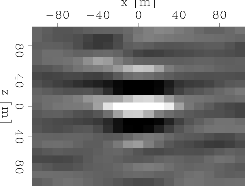
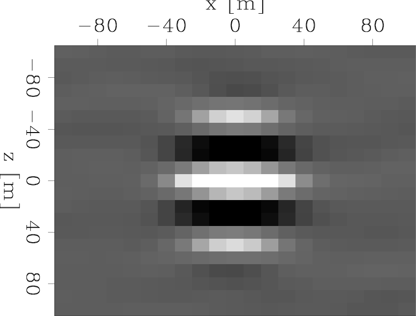
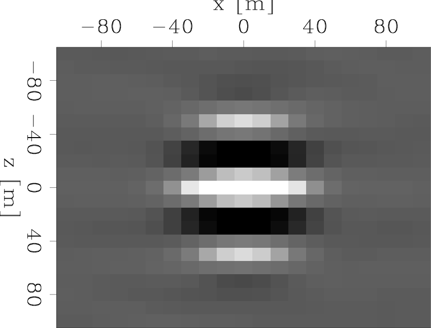
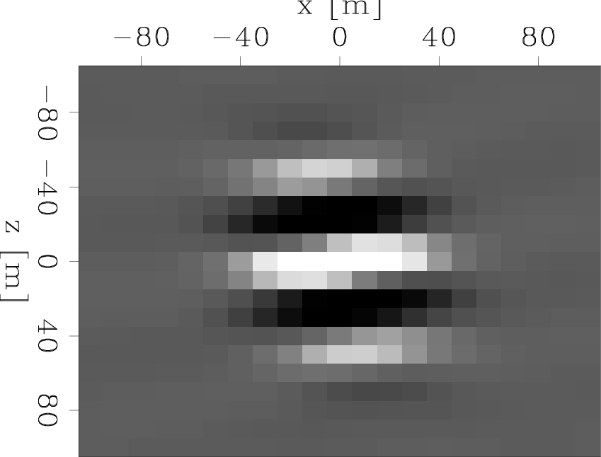
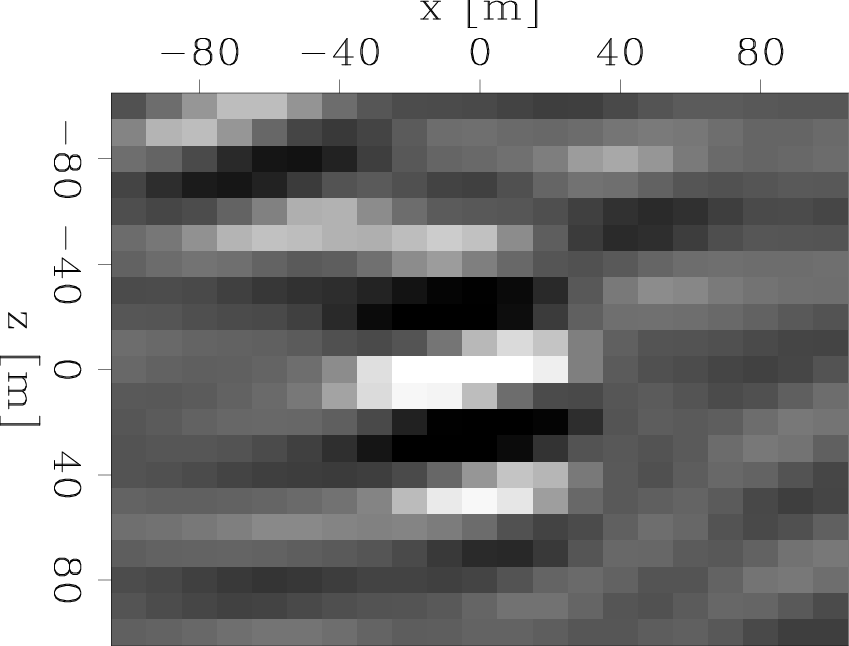
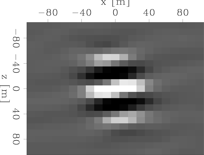
Figure 3
and 4 show the Hessian with
off-diagonals (with size
![]() ) obtained using different methods.
Figure 3 illustrates the result at image point
) obtained using different methods.
Figure 3 illustrates the result at image point
![]() ,
while Figure 4 illustrates the result at image point
,
while Figure 4 illustrates the result at image point
![]() .
These results also demonstrate that although simultaneous random phase encoding is efficient, the Hessian operator obtained by this method
(Figure 3(b) and Figure 4(b))
suffers a lot from unwanted crosstalk.
Encoding only the receiver-side Green's function with random phase functions gives accurate results
(Figure 3(d) and Figure 4(d));
however, the cost is similar to a shot-profile migration. In situations where the number of shot gathers is big, this encoding scheme may
not be a good choice. In contrast, the mixed phase-encoding scheme gives us very accurate results
(Figure 3(c) and Figure 4(c)) but with less cost than the
receiver-side encoded Hessian.
.
These results also demonstrate that although simultaneous random phase encoding is efficient, the Hessian operator obtained by this method
(Figure 3(b) and Figure 4(b))
suffers a lot from unwanted crosstalk.
Encoding only the receiver-side Green's function with random phase functions gives accurate results
(Figure 3(d) and Figure 4(d));
however, the cost is similar to a shot-profile migration. In situations where the number of shot gathers is big, this encoding scheme may
not be a good choice. In contrast, the mixed phase-encoding scheme gives us very accurate results
(Figure 3(c) and Figure 4(c)) but with less cost than the
receiver-side encoded Hessian.
|
|---|
|
hess-exact,hess-simul-random,hess-simul-mixed,hess-random
Figure 2. The diagonal of the Hessian obtained with different methods. Panel (a) is the exact diagonal of Hessian computed in the original shot-profile domain. Panel (b) is the result computed in the encoded source and receiver domain, where both the source and receiver Green's functions are randomly encoded. Panel (c) is the result also computed in the encoded source and receiver domain, where the source-side Green's functions are encoded with the plane-wave phase encoding function, while the receiver-side Green's functions are encoded with the random phase functions. Panel (d) is the result computed in the encoded receiver domain, where only the receiver-side Green's functions are randomly encoded. [CR] |
|
|

|
|---|
|
hess-exact-offd1,hess-simul-random-offd1,hess-simul-mixed-offd1,hess-random-offd1
Figure 3. The Hessian operator for an image point at |
|
|

|
|---|
|
hess-exact-offd2,hess-simul-random-offd2,hess-simul-mixed-offd2,hess-random-offd2
Figure 4. The Hessian operator for an image point at |
|
|
|
|
|
|
Modeling, migration, and inversion in the generalized source and receiver domain |