Modeling, migration, and inversion in the generalized source and receiver domain

Born modeling and inversion in the shot-profile domain

By using the Born approximation to the two-way wave equation, the primaries can be modeled by a linear operator as follows:

$$d({\bf x}_r,{\bf x}_s,\omega) = \sum_{\bf x}G({\bf x},{\bf x}_s,\omega)G({\bf x},{\bf x}_r,\omega)m({\bf x}),$$ (A-1)

where $d({\bf x}_r,{\bf x}_s,\omega)$ is the modeled data for a single frequency $\omega$ with source and receiver located at ${\bf x}_s=(x_s,y_s,0)$ and ${\bf x}_r=(x_r,y_r,0)$ on the surface; $G({\bf x},{\bf x}_s,\omega)$ and $G({\bf x},{\bf x}_r,\omega)$ are the Green's functions connecting the source and receiver, respectively, to the image point ${\bf x}=(x,y,z)$ in the subsurface; and $m({\bf x})$ denotes the reflectivity at image point ${\bf x}$. In Equation 1, we assume ${\bf x}_s$ and ${\bf x}_r$ are infinite in extent and independent of each other. For a particular survey, however, we do not have infinitely long cable and infinitely many sources; thus we have to introduce an acquisition mask matrix to limit the size of the modeling. We define

$$w({\bf x}_r,{\bf x}_s) = \left\{ \begin{array}{ll} 1 &\mbox{ if }... ...range of a shot at } {\bf x}_s; \\ 0 & \mbox{ otherwise }. \end{array} \right.$$ (A-2)

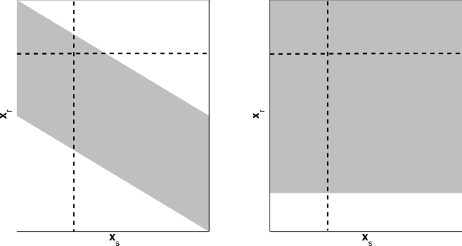
For the marine acquisition geometry, $w({\bf x}_r,{\bf x}_s)$ is similar to a band-limited diagonal matrix; for Ocean Bottom Cable (OBC) or land acquisition geometry, where all shots share the same receiver array, $w({\bf x}_r,{\bf x}_s)$ is a rectangular matrix. Figure 1 illustrates the acquisition mask matrices for these two typical geometries in 2-D cases.

acquisition-mask
Figure 1. Acquisition mask matrices for different geometries in 2-D cases. Greys denote ones while whites denote zeros. The left panel shows the acquisition mask matrix for a typical marine acquisition geometry; the right panel shows the acquisition mask matrix for a typical OBC or land acquisition geometry. [NR]

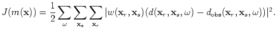
To find a model that best fits the observed data, we can minimize the following data-misfit function in the least-squares sense:

$$J(m({\bf x})) = \frac{1}{2}\sum_{\omega}\sum_{{\bf x}_s}\sum_{{\b... ...(d({\bf x}_r,{\bf x}_s,\omega)-d_{\rm obs}({\bf x}_r,{\bf x}_s,\omega))\vert^2.$$ (A-3)

The gradient of the above objective function gives the conventional shot-profile migration algorithm:

$$\nabla J({\b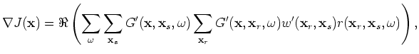f x}) = \Re \left( \sum_{\omega}\sum_{{\bf x}_s} G'({... ...\bf x}_r,\omega) w'({\bf x}_r,{\bf x}_s) r({\bf x}_r,{\bf x}_s,\omega) \right),$$ (A-4)

where $\Re$ denotes the real part of a complex number and $'$ means the complex conjugate; $r({\bf x}_r,{\bf x}_s,\omega)$ is the weighted residual defined as follows:

$$r({\bf x}_r,{\bf x}_s,\omega) = w({\bf x}_r,{\bf x}_s)(d({\bf x}_r,{\bf x}_s,\omega)-d_{\rm obs}({\bf x}_r,{\bf x}_s,\omega)).$$ (A-5)

The gradient or migration is only a rough estimate of the model $m({\bf x})$; to get a better recovery of the model space, the inverse of the Hessian, the second derivatives of the objective function, should be applied to the gradient:

$${\bf m} \approx {\bf H}^{-1}\nabla{\bf J}.$$ (A-6)

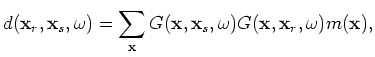
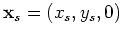
The Hessian can be explicitly constructed by taking the second-order derivatives of the objective function with respect to the model parameters as follows (Tang, 2008; Plessix and Mulder, 2004; Valenciano, 2008):

$$H({\bf x},{\bf y}) = \Re \left( \sum_{\omega} \sum_{{\bf x}_s} G({\bf x},{\bf x}_s,\omega)G'({\bf y},{\bf x}_s,\omega) \right. \times$$

$$\left. \sum_{{\bf x}_r} w^2({\bf x}_r,{\bf x}_s) G({\bf x},{\bf x}_r,\omega)G'({\bf y},{\bf x}_r,\omega)\right),$$ (A-7)

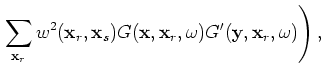where ${\bf y}$ is a neighbor point around the image point ${\bf x}$ in the subsurface.

Valenciano (2008) demonstrates that the Hessian can be directly computed using the above formula; however it requires storing a large number of Green's functions, which is inconvenient for dealing with large 3-D data set. Tang (2008) shows that with some minor alteration of Equation 7, an approximate Hessian can be efficiently computed using the phase-encoding method. However, Tang (2008) focuses more on the algorithm development, and the physics behind the Hessian by phase-encoding has not been carefully discussed. In this companion paper, I complete the discussion of the actual physics behind using phase-encoding methods, such as plane-wave phase encoding and random phase encoding, to obtain the Hessian. In the subsequent sections, I start with the modeling equation in the encoded source, encoded receiver and simultaneously encoded source and receiver domains. I show that the corresponding imaging Hessian in the generalized source and receiver domain is the same as those phase-encoded Hessians discussed in Tang (2008).

Modeling, migration, and inversion in the generalized source and receiver domain