Image-space wave-equation tomography in the generalized source domain

Numerical examples

We test the image-space wave-equation tomography in the generalized source domain on a simple model which contains only one reflector located at $z=1500$ m. Figure 1 shows the correct slowness model. The slowness model consists of a constant background slowness $1/2000$ s/m and two Gaussian anomalies located at $(x=-800,z=800)$ and $(x=800,z=800)$ respectively. The left anomaly has $5\%$ higher slowness, while the right one has $5\%$ lower slowness. We modeled $401$ shots ranging from $-4000$ m to $4000$ m, with a shot interval $20$ m. The receiver locations also range from $-4000$ m to $4000$ m, but with a $10$ m interval. The receivers are fixed for all shots to mimic a land acquisition geometry.

twin-slow
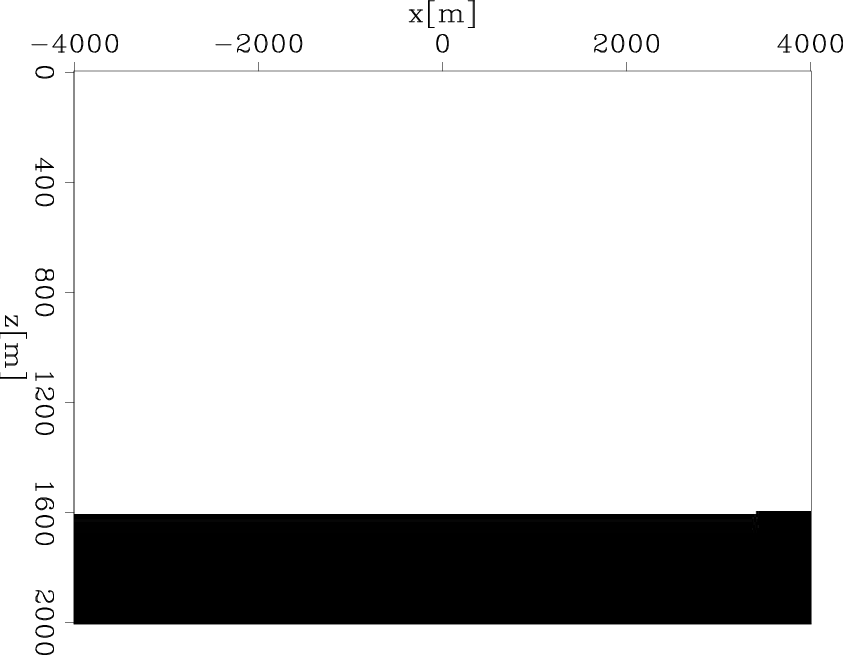
Figure 1. The correct slowness model. The slowness model consists of a constant background slowness ($1/2000$ s/m) and two $5\%$ Gaussian anomalies. [ER]

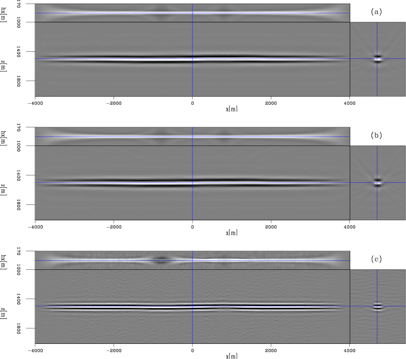
Figure 2 shows the migrated images in different domains computed with a background slowness $\widehat s = 1/2000$ s/m. Figure 2(a) is obtained by migrating the original $401$ shot gathers. Because of the inaccuracy of the slowness model, we can identify the mispositioning of the reflectors, especially beneath the Gaussian anomalies. Figure 2(b) is obtained by migrating the data-space plane-wave encoded gathers, where $61$ plane waves are migrated; the result is almost identical to that in Figure 2(a); Figure 2(c) is obtained by migrating the image-space encoded gathers. The image-space encoded areal source and receiver data are generated by simultaneously modeling $100$ randomly encoded unfocused SODCIGs, and $4$ realizations of the random sequence are used; hence we have $40$ image-space encoded areal gathers (each realization contains $10$ areal shots). The kinematics of the result look almost the same as those in Figure 2(a). However, notice the wavelet squeezing effect and the random noise in the background caused by the random phase encoding.

twin-bimg-all
Figure 2. Migrated image cubes with a constant background slowness ( $\widehat s = 1/2000$ s/m). Panel (a) is the result obtained in the original shot-profile domain; Panel (b) is the result obtained by migrating $61$ plane waves, while panel (c) is obtained by migrating $40$ image-space encoded areal gathers. [CR]

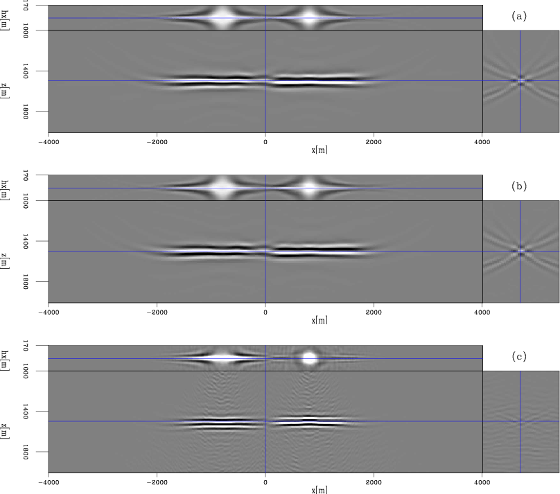
Figure 3 shows the image perturbations obtained by applying the forward tomographic operator ${\bf T}$ in different domains. For this example, we assume that we know the correct slowness perturbation $\Delta {\bf s}$, which is obtained by subtracting the background slowness $\widehat{\bf s}$ from the correct slowness ${\bf s}$. Figure 3(a) shows the image perturbation computed with the original $401$ shot gathers; notice the relative $90$ degree phase rotation compared to the background image shown in Figure 2(a). Figure 3(b) is the result obtained by using $61$ data-space plane-wave encoded gathers; the result is almost identical to Figure 3(a). Figure 3(c) shows the result computed with $40$ image-space encoded gathers; the kinematics are also similar to those in Figure 3(a).

twin-dimg-all
Figure 3. The image perturbations obtained by applying the forward tomographic operator ${\bf T}$ to the correct slowness perturbations in different domains. Panel (a) shows the image perturbation obtained using the original shot gathers, while panels (b) and (c) are obtained using the data-space encoded gathers and image-space encoded gathers, respectively. [CR]

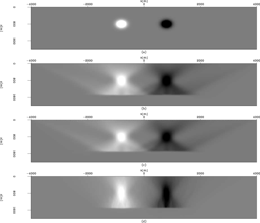
Figure 4 illustrates the predicted slowness perturbations by applying the adjoint tomographic operator ${\bf T}^{\prime }$ to the image perturbations obtained in Figure 3. For comparison, Figure 4(a) shows the correct slowness perturbation, i.e., $\Delta {\bf s} = {\bf s} - \widehat{\bf s}$; Figure 4(b) is the predicted slowness perturbation by back-projecting Figure 3(a) using all $401$ shot gathers; Figure 4(c) is the result by back-projecting Figure 3(b) using all $61$ data-space plane-wave encoded gathers and is almost identical to Figure 4(b); Figure 4(d) shows the result by back-projecting Figure 3(c) using all $40$ image-space encoded gathers. The result is also similar to Figure 4(b). However, notice that Figure 4(d) shows a slightly less focused result than Figure 4(b) and (c), which might be caused by the unattenuated crosstalk and the pseudo-random noise presented in Figure 3(c).

twin-dslw-all
Figure 4. The slowness perturbation obtained by applying the adjoint tomographic operator ${\bf T}^{\prime }$ on the image perturbations in Figure 3. Panel (a) shows the exact slowness perturbation; Panel (b) shows the slowness perturbation estimated by back-projecting the image perturbation shown in Figure 3(a); Panel (c) shows the result obtained using the data-space plane-wave encoded gathers by back-projecting Figure 3(b) and Panel (d) shows the result obtained using the image-space encoded gathers by back-projecting Figure 3(c). [CR]

The final example we show is the comparison among the gradients of the objective functional obtained in different domains. For simplicity, here we compare only the negative DSO gradients ( $-\nabla J_{\rm DSO}$) defined by Equation 8 (we compare $-\nabla J_{\rm DSO}$ instead of $\nabla J_{\rm DSO}$, because $-\nabla J_{\rm DSO}$ determines the search direction in a gradient-based nonlinear optimization algorithm). 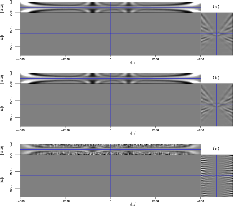Figure 5 shows the DSO image perturbations computed as follows:

$$\Delta {I}({\bf x},{\bf h}) = \vert{\bf h}\vert^2 \widehat {I}({\bf x},{\bf h}),$$ (A-38)

or in matrix form:

$$\Delta {\bf I} = {\bf O}^{\prime}{\bf O}\widehat{\bf I},$$ (A-39)

where ${\bf O}$ is the DSO operator. Figure 5(a) is the result obtained in the original shot-profile domain, whereas Figure 5(b) and (c) are obtained in the data-space phase-encoding domain and the image-space phase-encoding domain, respectively. The coherent energy at non-zero offests are indicators of velocity errors.

twin-dimg-offdso-all
Figure 5. The DSO image perturbations. The coherent energy at non-zero offsets indicates velocity errors. Panel (a) is obtained using the original shot gathers; Panels (b) and (c) are obtained using the data-space encoded gathers and the image-space encoded gathers, respectively. [CR]

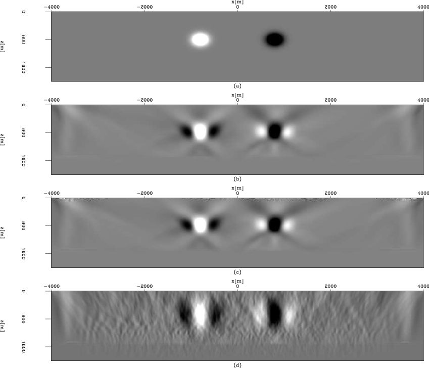
Figure 6 shows the negative gradients of the DSO objective functional ( $-\nabla J_{\rm DSO}$) obtained by back-projecting the DSO image perturbations shown in Figure 5. For comparison, Figure 6(a) shows the exact slowness perturbation, which is the same as Figure 4(a); Figure 6(b) shows the result obtained in the original shot-profile domain; Figure 6(c) shows the result obtained in the data-space phase-encoding domain, which is almost identical to Figure 6(b); Figure 6(d) shows the result obtained in the image-space phase-encoding domain. The result is also similar to Figure 6(b), though the unattenuated crosstalk and the random noise make the gradient less well behaved than those in Figure 6(b) and (c). Most important, the gradient in Figure 6(d) is pointing towards the correct direction, which is crucial for a gradient-based optimization algorithm to converge to the correct solution.

twin-dslw-offdso-all
Figure 6. The negative DSO gradients obtained using different methods. Panel (a) shows the exact slowness perurbation; Panel (b) shows the result obtained using the original shot gathers; Panels (c) and (d) show the results obtained using the data-space phase encoded gathers and the image-space phase encoded gathers, respectively. [CR]

Image-space wave-equation tomography in the generalized source domain