|
|
|
|
Seismic interferometry versus spatial auto-correlation method on the regional coda of the NPE |
 samples at a 125 Hz sampling frequency) at 610 stations with a 45-foot spacing. The second recording starts a few seconds after the first recording ends. Although the exact location of the NPE array is unknown, the data shows that the first 66 stations were located at an angle with respect to the other stations. Starting from station 67 located at
The spectrum at each station was estimated using a multitaper spectral-estimation technique. This provides several statistically independent estimates of the spectrum and decreases spectral leakage (Prieto et al., 2007,2008b). In this procedure, a time record with ![]() samples is first multiplied with a set of
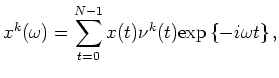
samples is first multiplied with a set of ![]() orthogonal Slepian tapers (Thomson, 1982). Second, the discrete Fourier transformation is computed for each tapered trace as follows:
orthogonal Slepian tapers (Thomson, 1982). Second, the discrete Fourier transformation is computed for each tapered trace as follows:
| (12) |
 Slepian taper is denoted by
 | (13) |
 . To enhance the signal-to-noise ratio, the retrieved gathers are smoothed over 50 midpoints, corresponding to a length of
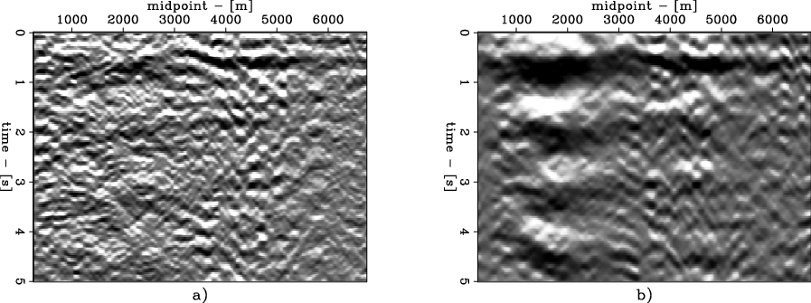
We first study the result from processing the records in the time domain, as is common in seismic interferometry practices. A common-midpoint section at
![]() is given in Figure 4, and a common-offset section for
is given in Figure 4, and a common-offset section for
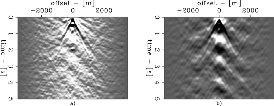
![]() is given in Figure 5. de Ridder (2008) did not observe any event, besides the surface-wave events intersecting each other at
is given in Figure 5. de Ridder (2008) did not observe any event, besides the surface-wave events intersecting each other at
![]() that is coherent across different midpoints. When we study the common-offset section in Figure 5, we can see the arrival time of the surface wave event at
that is coherent across different midpoints. When we study the common-offset section in Figure 5, we can see the arrival time of the surface wave event at
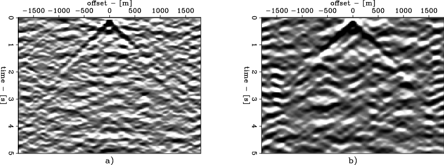
![]() slightly varying with offset. If we neglect this and assume the earth is horizontally layered, the recovered gathers can be stacked over common-offsets as shown in Figure 6. Estimating the slope of the event visible in Figures 4 and 6, de Ridder (2008) found a velocity of
slightly varying with offset. If we neglect this and assume the earth is horizontally layered, the recovered gathers can be stacked over common-offsets as shown in Figure 6. Estimating the slope of the event visible in Figures 4 and 6, de Ridder (2008) found a velocity of
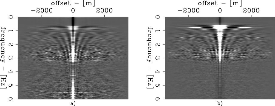
![]() . The subscript
. The subscript ![]() refers to a Rayleigh wave, which is the dominant surface-wave type recorded in the vertical component of particle velocity in groundroll. It is difficult to extract more information from the time-domain images. Additional analysis of the retrieved gathers can be performed in the frequency-domain, by inverting for phase velocity and attenuation factors. The frequency-domain equivalents of the time-domain gathers in Figures 4 and 6 are shown respectively in Figures 7 and 9.
refers to a Rayleigh wave, which is the dominant surface-wave type recorded in the vertical component of particle velocity in groundroll. It is difficult to extract more information from the time-domain images. Additional analysis of the retrieved gathers can be performed in the frequency-domain, by inverting for phase velocity and attenuation factors. The frequency-domain equivalents of the time-domain gathers in Figures 4 and 6 are shown respectively in Figures 7 and 9.
|
|---|
|
si375m
Figure 4. Interferometric common-midpoint gather gather, at |
|
|
|
|---|
|
si375o
Figure 5. Interferometric common-offset gather, for |
|
|
|
|---|
|
SIHS
Figure 6. Common-offset stack for the interferometric gathers; a) retrieved from recording 1, b) retrieved from recording 2. [ER] |
|
|
|
|---|
|
SPACHS
Figure 7. Frequency-domain common-offset stack; a) retrieved from recording 1, b) retrieved from recording 2. [ER] |
|
|
|
|
|
|
Seismic interferometry versus spatial auto-correlation method on the regional coda of the NPE |