|
|
|
|
Angle-domain common-image gathers in generalized coordinates |
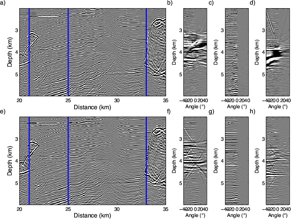
Figure 7 shows slices all clipped at the 99![]() percentile from the corresponding elliptic and Cartesian ADCIG image volumes.
percentile from the corresponding elliptic and Cartesian ADCIG image volumes.
|
|---|
|
GOOD
Figure 7. Vertical elliptic and Cartesian ADCIGs slices using the correct migration velocity model. a) Elliptic coordinate image with three vertical lines showing the locations of ADCIG gathers from left to right in panels b-d. e) Cartesian coordinate image with three vertical lines showing the locations of ADCIG gathers from left to right in panels f-h. |
|
|
The image in panel 7d has a wide reflection zone between 3.75-4.25 km in depth, which occurs because the shown angle gather is a vertical slice through the nearly vertical salt flank. This creates the appears of low-frequency noise, which is the appropriate response for a near-vertical reflector. Panel 7e shows the Cartesian image for the same location as panel 7a, while panels 7f-h are extracted from the same locations as panels 7b-d. The Cartesian angle gathers look similar to those in elliptic coordinates, except for the salt flanks to the right-hand-side of panel 7h.
A final observation from Figure 7 is that ADCIGs calculated via subsurface correlations will generate artifacts at locations near salt-sediment interfaces - whether in an elliptic or a Cartesian coordinate system. This geologic setting leads to situations where a wavefield sample inside a salt body is correlated with another sample located in the sediment with a significantly different velocity. This velocity difference violates one of the theoretical ADCIG assumptions, namely that the velocity remains constant across the correlation window. Hence, one must be careful not to interpret ADCIG artifacts as signal useful for migration velocity analysis.
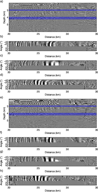
Figure 8 shows horizontal slices that better resolve the vertical salt flank. Panel 8a presents the elliptic coordinate image, with three horizontal lines showing the ADCIG slice locations from top to bottom. The right-hand sides of panels 8b-d display the well-focused vertical salt-flank reflector. This demonstrates the robustness of the ADCIG calculation in elliptic coordinates.
|
|---|
|
GOODZ
Figure 8. Horizontal elliptic and Cartesian ADCIGs slices using the correct migration velocity model. a) Elliptic coordinate image with three horizontal lines showing the locations of horizontal ADCIG gathers from top to bottom in panels b-d. e) Cartesian coordinate image with three horizontal lines showing the locations of horizontal ADCIG gathers from top to bottom in panels f-h. |
|
|
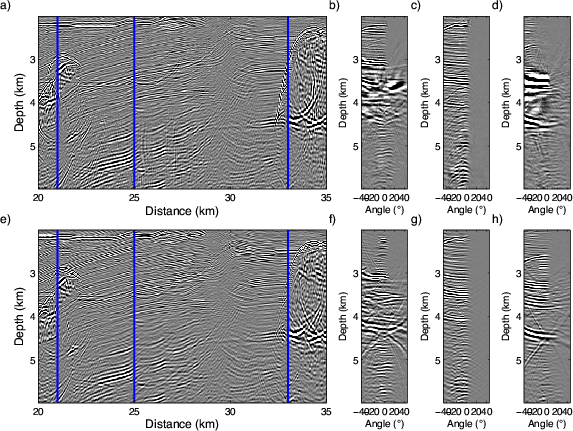
An additional test examines how the ADCIG volumes change when introducing an incorrect migration velocity profile. Figure 9 presents ADCIG volumes similar to those shown in Figure 7 after using a migration velocity profile rescaled by 98%.
|
|---|
|
BAD
Figure 9. Vertical elliptic and Cartesian ADCIGs slices using an incorrect migration velocity model. a) Elliptic coordinate image with three vertical lines showing the locations of vertical ADCIG gathers from left to right in panels b-d. e) Cartesian coordinate image with three vertical lines showing the locations of vertical ADCIG gathers from left to right in panels f-h. |
|
|
|
|---|
|
BADZ
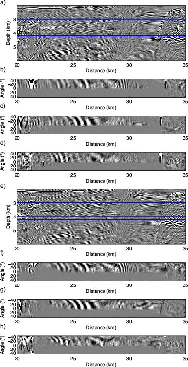
Figure 10. Horizontal elliptic and Cartesian ADCIGs slices using an incorrect migration velocity model. a) Elliptic coordinate image with three horizontal lines showing the locations of horizontal ADCIG gathers from top to bottom in panels b-d. e) Cartesian coordinate image with three horizontal lines showing the locations of horizontal ADCIG gathers from top to bottom in panels f-h. |
|
|
|
|
|
|
Angle-domain common-image gathers in generalized coordinates |