 |
 |
 |
 | Joint wave-equation inversion of time-lapse seismic data |  |
![[pdf]](icons/pdf.png) |
Next: Joint-inversion
Up: Theory
Previous: Theory
Given a linear modeling operator  , the seismic data
  can be computed as
 |
(A-1) |
where  is the reflectivity model. The modeling operator, , in this study, represents the seismic acquisition process.
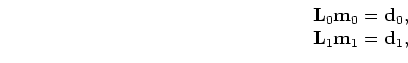
Two different surveys -- say a baseline and monitor -- acquired at different times (
is the reflectivity model. The modeling operator, , in this study, represents the seismic acquisition process.
Two different surveys -- say a baseline and monitor -- acquired at different times ( and
and  respectively) over the same earth model can be represented as follows:
 |
(A-2) |
where
 and
and
 are respectively the reflectivity models at the times when the datasets
 and
and
 were acquired, and
 and
and
 are the modeling operators defining the acquisition process for the two surveys (baseline and monitor).
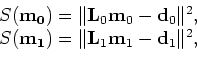
The quadratic cost functions for equation 2 are given by
 |
(A-3) |
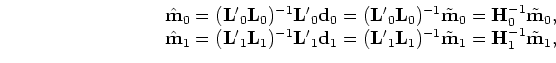
and the least-squares solutions are
 |
(A-4) |
where
 and
and
 are the migrated baseline and monitor images,
 and
and
 are the inverted images,
 and
and
 are the migration operators (adjoints to the modeling operators
and
respectively), and
are the migration operators (adjoints to the modeling operators
and
respectively), and
 and
and
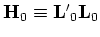 , are the Hessian matrices.
Here, and in other parts of this paper, the symbol
, are the Hessian matrices.
Here, and in other parts of this paper, the symbol 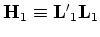 denotes transposed complex conjugate.
These formulations are based on (but not limited to) one-way wave-equation extrapolation methods.
denotes transposed complex conjugate.
These formulations are based on (but not limited to) one-way wave-equation extrapolation methods.
The Hessian matrices are the second derivatives of the cost functions (equation 3) with respect to all model points in the image.
Because the Hessian matrices are generally not invertible for almost any practical scenario, equation 4 is solved iteratively as follows:
 |
(A-5) |
An inverted time-lapse image,
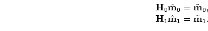 , can be obtained as the difference between the two images,
and
, obtained from equation 5:
, can be obtained as the difference between the two images,
and
, obtained from equation 5:
 |
(A-6) |
We will refer to the method of computing the time-lapse image using equation 6 as 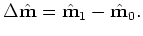
 throughout the rest of this paper.
|
|
|
|
| Joint wave-equation inversion of time-lapse seismic data | |
|
Next: Joint-inversion
Up: Theory
Previous: Theory
2009-04-13