Angle domain common image gathers for steep reflectors

Numerical examples

We apply both reverse-time migration and plane-wave migration in tilted coordinates on the BP velocity benchmark dataset (Billette and Brandsberg-Dahl, 2005). Figure 1 shows the velocity model of the dataset. The maximum offset is $15$ km, which is much larger than that in a realistic case. We mainly focus on the area from $x=20$ km to $x=35$ km. Figure 2 shows the image of that area obtained by plane-wave migration in tilted coordinates. In this area, there are both steep salt flanks and near-flat sediments. We run migration with both the true velocity and the velocity that is 3 percent slower than the true one. We start with showing examples that both horizontal and vertical CIGs of reverse-time migration are not robust where there are a full-range of dip directions. Then we compare angle domain CIGs of plane-wave migration in tilted coordinates with those of reverse-time migration obtained by merging the horizontal and vertical CIGs.

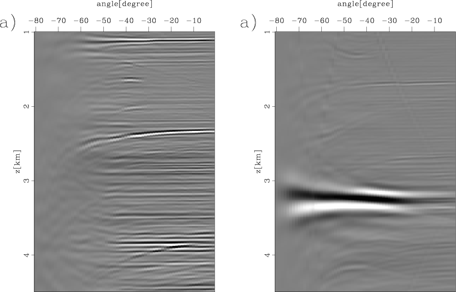
axgathers Figure 5. Horizontal angle domain CIGs with the true velocity obtained by reverse-time migration. (a) For the near-flat sediments at $x=23$ km, the gathers are flat except the multiples. (b) For the steep salt flank at $33.2$ km, the gathers are smeared because of the horizontal-offset stretch.

azgather
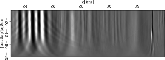
Figure 6. Vertical angle domain CIGs with the true velocity obtained by reverse-time migration. The CIGs of the sediments at $x=24.5$ km are smeared and the CIGs for the salt flank are at the same horizontal location for all angles.

Figure 3 shows the horizontal subsurface offset domain CIGs with the true velocity obtained by reverse-time migration. Figure 3(a) shows the horizontal offset domain CIGs of the near-flat sediments at $x=23$ km. The energy mostly focuses well at zero offset. Notice that the multiple energy (at $z=2.3$ km and $z=3.9$ km) does not focus at zero offset. Figure 3(b) shows the horizontal offset domain CIGs of the steep salt flank at $x=33.2$ km. The energy leaks to far offsets because of the stretch of the horizontal subsurface offset at steep reflectors. Figure 4 shows the vertical subsurface offset domain CIGs at $z=3.25$ km. For the steep salt flank at $x=33.2$ km, the energy focuses well at zero offset while the energy leaks to far offsets for the near-flat sediments at $x=24.5$ km. As in the theoretical analysis, horizontal offset domain CIGs are good for near-flat reflectors while vertical ones are good for steep reflectors.

Figures 5 and 6 show the horizontal and vertical angle domain CIGs with the true velocity obtained by reverse-time migration, respectively. Figure 5(a) shows the horizontal angle domain CIGs of near-flat sediments at $x=23$ km. The gathers are flat since we use the true velocity in migration. Notice that the gathers of multiples bend down at $z=2.3$ km and $z=3.9$ km. Figure 5 (b) shows the horizontal angle domain CIGs of the steep salt flank at $x=33.2$ km. The horizontal gathers of the salt flank look smeared because of the offset stretch. In contrast, in Figure 6 the vertical angle domain CIGs of the steep salt flank (at $x=33.2$ km) are at the same horizontal location for all angles but those of the near-flat sediments ($x=24.5$ km) look smeared.

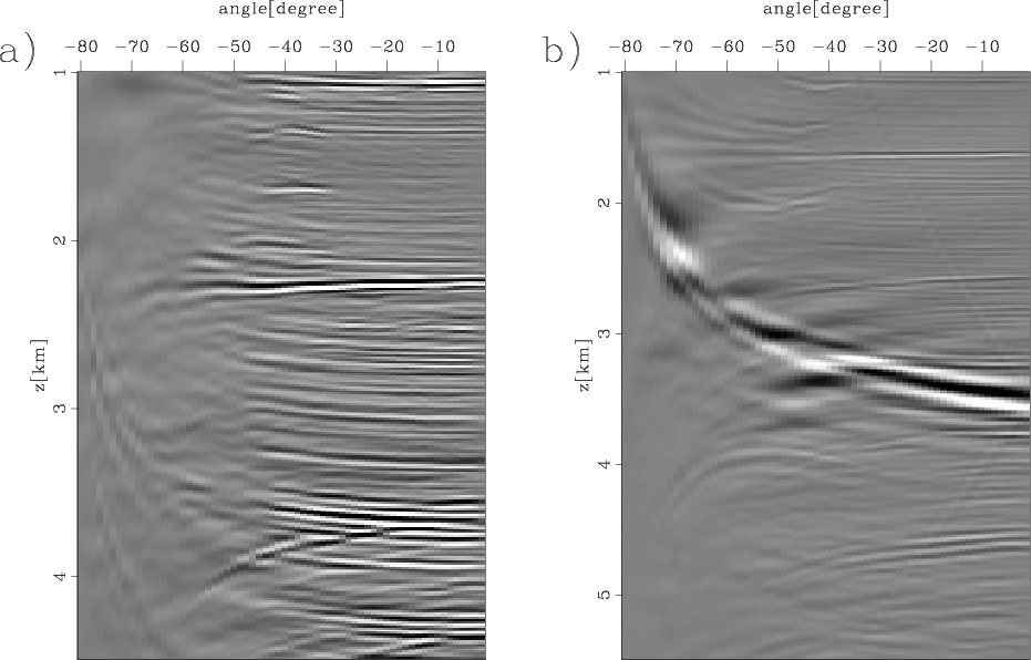
ax97gathers Figure 7. Horizontal angle domain CIGs with the 3 percent slower velocity obtained by reverse-time migration. (a) For the near-flat sediments at $x=23$ km, the gathers show reasonable curvature. (b) For the steep salt flank at $x=33.2$ km, the gather is a little smeared. The moveout is not reasonable, given the 3 percent velocity error.

az97gather
Figure 8. Vertical angle domain CIGs with the 3 percent slower velocity obtained by reverse-time migration. The gather of the salt flank at $x=33$ km shows reasonable moveout. The gathers of the sediments at $x=30.5$ km look smeared.

cigtruertm
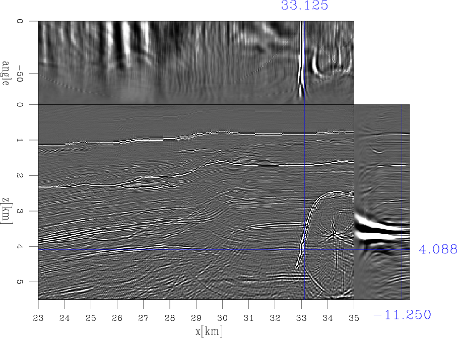
Figure 9. Angle domain CIG cube with the true velocity obtained by reverse-time migration.

cigtruetilt
Figure 10. Angle domain CIG cube with the true velocity obtained by plane-wave migration in tilted coordinates.

Figures 7 and 8 show a migration with the 3 percent slower velocity in the horizontal and vertical angle domain CIGs, respectively. The horizontal location for Figure 7(a) and (b) are at $x=23$ km and $x=33.2$ km, respectively. And the vertical location for Figure 8 is at $z=3.5$ km. The horizontal angle domain CIGs for the sediments bend up with reasonable moveouts in Figure 7(a), but the horizontal angle domain CIGs for the salt flank look smeared in Figure 7(b). The moveout in the CIGs of the salt flank is too large given the 3 percent velocity error. In contrast, in Figure 8 the moveout in the vertical angle domain CIGs of the salt flank (at $x=33$ km) is reasonable, but the vertical CIGs of sediments at $x=30.5$ km look smeared in Figure 8.

stack
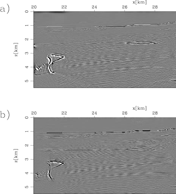
Figure 11. Stack images from angle domain CIGs with the true velocity: (a) reverse-time migration; (b) plane-wave migration in tilted coordinates.

As with the theoretical analysis, Figures 3 to 8 demonstrate that in reverse-time migration both horizontal and vertical CIGs are not robust in complex area, where there are reflectors with a full range of dip. To obtain reliable CIGs, we merge horizontal and vertical angle domain CIGs by applying equation 8. We can also obtain reliable CIGs by plane-wave migration in tilted coordinates. In the previous section, we discussed two ways to generate angle domain CIGs in plane-wave migration in tilted coordinates. We choose the former one for the following examples. We transform offset domain CIGs into angle domain CIGs in tilted coordinates and then rotate the angle domain CIGs back to vertical Cartesian coordinates. Figures 9 to 12 compare the angle domain CIGs obtained by reverse-time migration and plane-wave migration in tilted coordinates.

After 2-D migration, angle domain CIGs are a 3-D cube $I(x,z,\gamma)$. Conventionally, we look at vertical sections of the cube $I(x=x_0,z,\gamma)$. However, the image point moves along the direction normal to the apparent geologic dip of the reflector when the velocity is not correct (Biondi and Symes, 2004). Therefore, the CIG of a image point should be viewed in the direction normal to its apparent geologic dip. Otherwise, for a steeply dipping reflectors, if we still look at the CIG cube in a vertical direction, most of the energy in the CIG we see belongs to image points in its neighborhood.

amerg9770
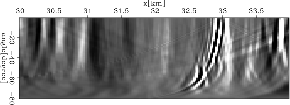
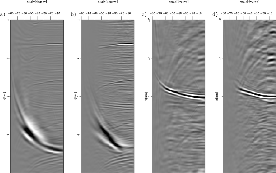
Figure 12. The angle CIGs with the 3 percent slower velocity. (a) The vertical view of angle domain CIGs obtained by reverse-time migration at $x=32.6$ km. (b) The vertical view of angle domain CIGs obtained by plane-wave migration in tilted coordinates at $x=32.6$ km. (c) The normal-direction view of angle domain CIGs obtained by reverse-time migration at $x=32.6$ km, $z=4.4$ km. (d) The normal-direction view of angle domain CIGs obtained by plane-wave migration in tilted coordinates at $x=32.6$ km, $z=4.4$ km.

Figures 9 and 10 respectively show the CIG cubes with the true velocity obtained by reverse-time migration and plane-wave migration in tilted coordinates. In both figures, the top panel shows the CIGs in the horizontal direction and the side panel shows the CIGs in the vertical direction. Reverse-time migration has better large-angle energy compared to plane-wave migration in tilted coordinates, but otherwise they are comparable. The offset of this dataset is unrealistically large and thus the maxmum opening angle is unrealistically large. Plane-wave migration in tilted coordinates is still based on the one-way wave equation. Both source and receiver wavefields are extrapolated in the same coordinates, so when opening angle is very large (more than $60^\circ$ ), the angle difference of source and receiver rays is large and thus one of them cannot be modeled accurately. But there is no angle limitation in reverse-time migration, therefore its large-angle energy are better handled than plane-wave migration in tilted coordinates. Given the realistic offset in real datasets, opening angles are usually smaller than $50^\circ$. Therefore, angle domain CIGs of the two migrations are comparable for a real dataset. Notice that in both figures the CIGs of the steep salt flank look smeared in the side panel and those of the sediments look smeared in the top panel. This demonstrates that angle domain CIGs should be viewed in the direction normal to the dip direction. Figure 11 compares the stacks of the angle domain CIGs along the angle axis. Figure 11(a) is obtained by reverse-time migration and Figure 11(b) is obtained by plane-wave migration in tilted coordinates and the images are comparable.

Figure 12 shows the comparison of angle domain CIGs with the velocity that is 3 percent slower than the true one. Figures 12(a) and (b) are the vertical views of the angle domain CIGs obtained by reverse-time migration and plane-wave migration in tilted coordinates, respectively. The horizontal location for them is at $x=32.6$ km, where there are near-flat sediments at the shallow part and steep salt flanks at $z=4.4$ km. The events bending down are multiples. As with the CIGs with the true velocity, reverse-time migration has better far-angle energy compared to plane-wave migration in tilted coordinates. In both figures, the moveout of the CIGs of the sediments is reasonable because the viewing direction is almost normal to their apparent geologic dip direction. But the CIGs of the salt flank (at $z=4.4$ km) look smeared and forked because the viewing direction almost parallels its dip and most far-angle energy in the CIG belongs to the image points in its neighborhood. The curvature of the CIG is not reasonable and the moveout is too large, given the 3 percent velocity error.

Figures 12(c) and (d) are the normal-direction view of the angle domain CIGs obtained by reverse-time migration and plane-wave migration in tilted coordinates, respectively. The location of the event is at $x=32.6$ km, $z=4.4$ km, where the salt flank is present. Its apparent geologic dip is about $70^\circ$. The vertical axis in both panels is the direction normal to the apparent geologic dip of the reflector. Similarly, reverse-time migration has better far-angle energy, otherwise Figures 12(c) and (d) are comparable. Given the 3 percent velocity error, both the CIGs show a reasonable curvature.

Angle domain common image gathers for steep reflectors