Ground-roll

As a final example, consider the problem of separating spatially-aliased ground-roll from body waves in land data. This a more challenging application of the algorithm because the body waves have curvature that changes rapidly with both offset and time so to match it I need small filters in relatively small patches. The ground-roll, on the other hand, has little global curvature (although it may have strong local curvature due to aliasing) and matching it is more successful with large filters in large patches. A refinement to the method could use different regularization operators or at least different regularization parameters $\epsilon$ on the non-stationary filters for the primaries and the multiples. For the sake of simplicity, I used the same regularization for both.

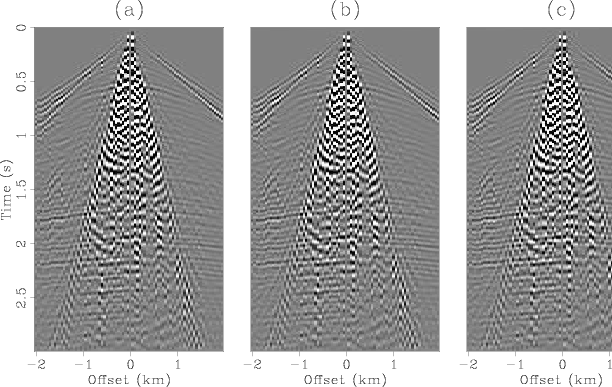
Figure 15 shows the original shot as well as the initial estimates of the body waves and the ground-roll. The ground-roll estimate was computed simply by high-cut filtering the data to 24 Hz using a Butterworth filter with six poles. I allowed significant energy from the body waves to leak into the estimate of the ground-roll to illustrate the problem described in the previous paragraph. Similarly, the estimate of the body waves was computed by low-cut filtering the data to 18 Hz also with a Butterworth filter with 6 poles. Since I don't want to reduce the low frequency components of the signal too much, I allowed strong ground-roll to leak into the estimate of the body waves. The purpose is to eliminate this ground-roll without hurting the signal and ideally, mapping back some of the body-waves from the estimate of the ground-roll.

shot1-estimates1
Figure 15. Land shot gather with strong ground-roll (a), initial estimate of ground-roll (b), and body waves (c).

shot1-matched-bw
Figure 16. Estimate of body waves after one outer iteration (a), after 5 outer iterations (b) and after 10 outer iterations (c). Notice how after the fifth iteration the ground-roll is essentially gone.

shot1-matched-gr
Figure 17. Estimate of ground-roll after one outer iteration (a), after 5 outer iterations (b) and after 10 outer iterations (c). Some of the body waves have been removed in panel (c) but much still remains.

Figure 16 shows the estimate of the body-waves after one, five and 10 outer iterations of the proposed algorithm. Even after just the first iteration, most of the ground-roll has been eliminated and after five iterations it is almost gone. For this example I used just two patches in time and one in offset. Figure 17 shows similar results for the ground-roll. Since the patches were so large, the energy of the leaked body-waves were only slightly attenuated (see the reflector at about 1.7 secs). This energy was mapped back to the estimate of the body-waves.