

Next: Conclusions and future work
Up: Lomask and Guitton: Flattening
Previous: The L-BFGS-B algorithm
We conducted preliminary tests of these modified flattening methods on
both 2D and 3D data sets from the Gulf of Mexico and the North Sea,
respectively. We only show the results obtained with the Gauss-Newton
approach, the L-BFGS-B results being almost identical.
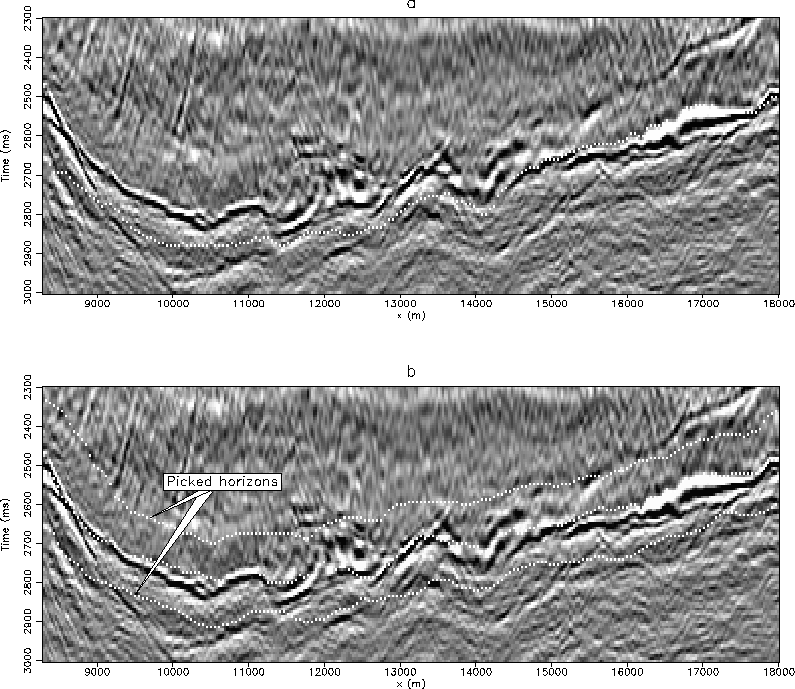
In the top of Figure ![[*]](http://sepwww.stanford.edu/latex2html/cross_ref_motif.gif) is an image of the lower portion of a salt boundary from the Gulf of Mexico. Overlain on this image is a single horizon that results from the unconstrained flattening method. The horizon fails to track the boundary accurately. In the lower image, two picked horizons have been added as hard constraints. Notice that the center horizon now does an overall much better job of tracking the boundary than its unconstrained counterpart. Unfortunately, the price paid is that by applying regularization in time, the constrained horizon does not track the character of data locally as well.
is an image of the lower portion of a salt boundary from the Gulf of Mexico. Overlain on this image is a single horizon that results from the unconstrained flattening method. The horizon fails to track the boundary accurately. In the lower image, two picked horizons have been added as hard constraints. Notice that the center horizon now does an overall much better job of tracking the boundary than its unconstrained counterpart. Unfortunately, the price paid is that by applying regularization in time, the constrained horizon does not track the character of data locally as well.
GoM_combo
Figure 1 Images of a 2D Gulf of Mexico data set with flattening picks overlaying a salt boundary: (a) unconstrained, (b) with the upper and lower picked horizons as hard constraints. Notice that the middle horizon in (b) tracks the boundary more accurately than its unconstrained counterpart in (a).


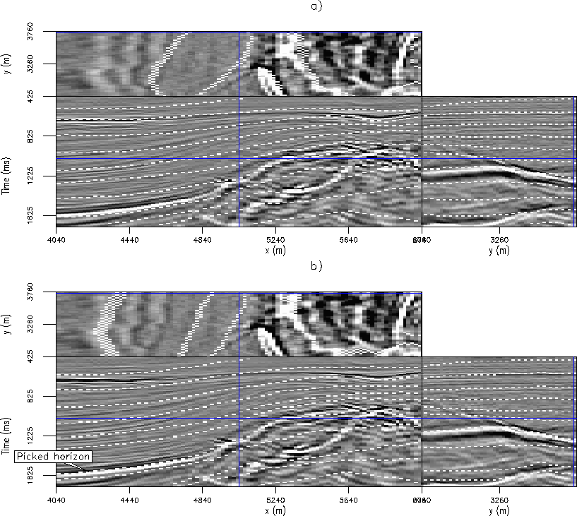
In Figure ![[*]](http://sepwww.stanford.edu/latex2html/cross_ref_motif.gif) is a 3D North Sea data set. The top shows several horizons that result from unconstrained flattening. Although some of the horizons are well tracked, several are not. In the lower figure, we picked the brightest horizon and passed it into the flattening method as a hard constraint. Notice that the reflectors above it now tend to more accurately track their respective events.
is a 3D North Sea data set. The top shows several horizons that result from unconstrained flattening. Although some of the horizons are well tracked, several are not. In the lower figure, we picked the brightest horizon and passed it into the flattening method as a hard constraint. Notice that the reflectors above it now tend to more accurately track their respective events.
Also in Figure ![[*]](http://sepwww.stanford.edu/latex2html/cross_ref_motif.gif) , notice how the reflectors at the top of the cube are tracked more accurately without constraints. This is as expected because the regularization is causing the reflectors to conform to one another. To mitigate this, we could have passed an upper picked horizon from the unconstrained result as an additional hard constraint to the lower result.
, notice how the reflectors at the top of the cube are tracked more accurately without constraints. This is as expected because the regularization is causing the reflectors to conform to one another. To mitigate this, we could have passed an upper picked horizon from the unconstrained result as an additional hard constraint to the lower result.
elf_pck3_combo
Figure 2 Images of a 3D North Sea data set with flattening picks: (a) unconstrained, (b) with a single picked horizon as a hard constraint. Notice that with the hard constraint, reflectors near the picked horizon are tracked more accurately.


Next: Conclusions and future work
Up: Lomask and Guitton: Flattening
Previous: The L-BFGS-B algorithm
Stanford Exploration Project
4/6/2006
![[*]](http://sepwww.stanford.edu/latex2html/cross_ref_motif.gif) is an image of the lower portion of a salt boundary from the Gulf of Mexico. Overlain on this image is a single horizon that results from the unconstrained flattening method. The horizon fails to track the boundary accurately. In the lower image, two picked horizons have been added as hard constraints. Notice that the center horizon now does an overall much better job of tracking the boundary than its unconstrained counterpart. Unfortunately, the price paid is that by applying regularization in time, the constrained horizon does not track the character of data locally as well.
is an image of the lower portion of a salt boundary from the Gulf of Mexico. Overlain on this image is a single horizon that results from the unconstrained flattening method. The horizon fails to track the boundary accurately. In the lower image, two picked horizons have been added as hard constraints. Notice that the center horizon now does an overall much better job of tracking the boundary than its unconstrained counterpart. Unfortunately, the price paid is that by applying regularization in time, the constrained horizon does not track the character of data locally as well.

