Preconditioning with the helical derivative

We can reduce the computation time significantly by preconditioning by substituting $\boldsymbol{\boldsymbol{\tau}} = {\bf H}^{-1} {\bf m}$, where ${\bf H}^{-1}$ is the inverse of the 3D helical derivative Claerbout (1999). Preconditioning with the helical derivative is a logical choice because its inverse is very close to the inverse of a gradient. However, recall that our 3D gradient operator $\boldsymbol{\nabla}_\epsilon$ is actually a chain of two matrices ${\bf W}_\epsilon$ and $\boldsymbol{\nabla}$. Instead of approximating the inverse of $(\boldsymbol{\nabla}^T\boldsymbol{\nabla})^{-1}$, we wish to approximate the inverse of $(\boldsymbol{\nabla}^T {{\bf W}_\epsilon}^2 \boldsymbol{\nabla})^{-1}$. Therefore, we factor the finite difference approximation to the Laplacian with an $\epsilon$ parameter. In 2D, we factor the Laplacian with an epsilon parameter as:  

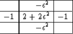$$\quad \quad \begin{array} {\vert r\vert r\vert r\vert} \hlin... ...+2\epsilon^2 & -1\ \hline & -\epsilon^2 & \ \hline\end{array}$$ (16)

To extend to 3D, we add another 2 to the center and another set of -1's in the 3rd dimension. Once factored it becomes a 3D helical derivative ${\bf H}_\epsilon$ with a scalar weight, $\epsilon$, applied to the time(or depth) axis. When used as a regularization operator, this has the desirable property of having only one output. We choose not to include the mask $\bf K$ in the preconditioner because it is non-stationary.

With preconditioning, equation (13) becomes this:  

$$\bold r \quad = \quad \boldsymbol{\nabla}_\epsilon\bold K {{... ... m} - {\bf p}(x,y,\boldsymbol{\boldsymbol{\tau}}_k)+ \bold r_0.$$ (17)

We pay a significant price in memory cost for this computational time saving. To precondition this equation requires chaining together several operators thus several temporary arrays are allocated. Also, the computational expense is tied to the number of coefficients used in the filter which in 3D is typically 20.