 |
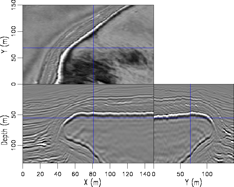
Figure 3 A Gulf of Mexico 3D data set with a prominent salt boundary.
 |
 |
 |
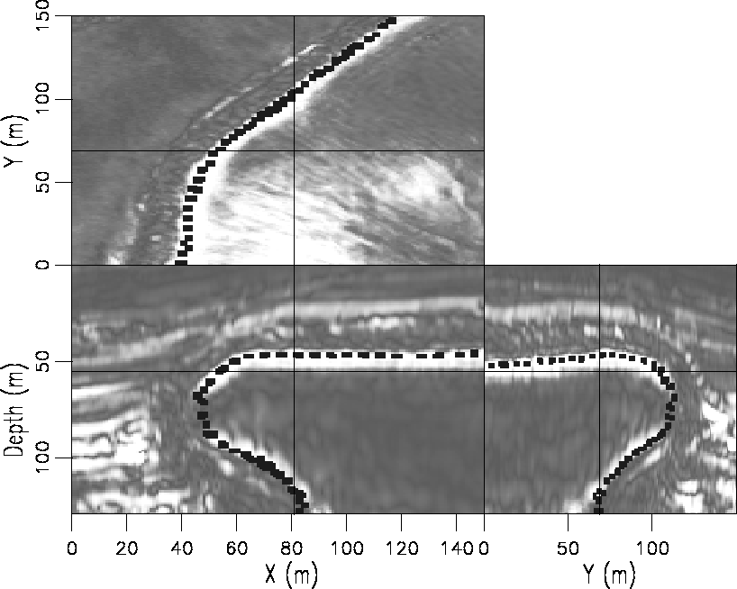 |
![[*]](http://sepwww.stanford.edu/latex2html/cross_ref_motif.gif) and overlain on the instantaneous amplitude of data. It accurately tracks the boundary.
and overlain on the instantaneous amplitude of data. It accurately tracks the boundary.
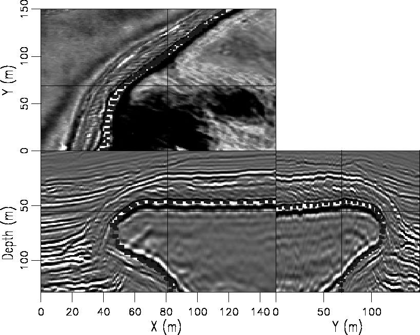 |
![[*]](http://sepwww.stanford.edu/latex2html/cross_ref_motif.gif) except the boundary is overlain on the data itself. Notice it accurately tracks the boundary except where the amplitude is weak. It also has difficulty at the boundary of the image itself.
except the boundary is overlain on the data itself. Notice it accurately tracks the boundary except where the amplitude is weak. It also has difficulty at the boundary of the image itself.
In Figure ![[*]](http://sepwww.stanford.edu/latex2html/cross_ref_motif.gif) is a 3D seismic cube from the offshore with a prominent salt boundary. Figure
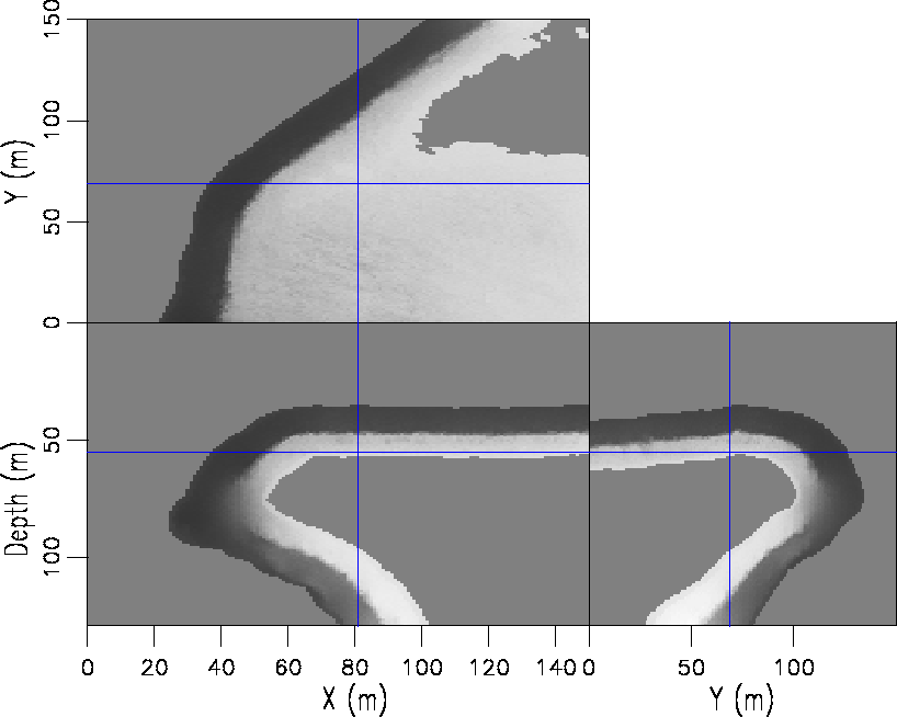
is a 3D seismic cube from the offshore with a prominent salt boundary. Figure ![[*]](http://sepwww.stanford.edu/latex2html/cross_ref_motif.gif) shows the mask used to define the bounds. In this case, we used the velocity model to define the upper and lower bounds. Alternatively, we could have garnered the bounds from a first pass on a sub-sampled cube.
shows the mask used to define the bounds. In this case, we used the velocity model to define the upper and lower bounds. Alternatively, we could have garnered the bounds from a first pass on a sub-sampled cube.
The second smallest eigenvector from the method is displayed in Figure ![[*]](http://sepwww.stanford.edu/latex2html/cross_ref_motif.gif) . The eigenvector is split along the salt boundary rather than along its shorted dimension as would have resulted without random bounds. Figure
. The eigenvector is split along the salt boundary rather than along its shorted dimension as would have resulted without random bounds. Figure ![[*]](http://sepwww.stanford.edu/latex2html/cross_ref_motif.gif) displays the envelope of the data with the resulting salt boundary pick overlaying it. Notice it does a good job of tracking the peak of the amplitude. This illustrates that our method can be applied to 3D cubes. This is not surprising as the method has already been applied successfully to 3D atomic meshes Hale and Emanuel (2003).
displays the envelope of the data with the resulting salt boundary pick overlaying it. Notice it does a good job of tracking the peak of the amplitude. This illustrates that our method can be applied to 3D cubes. This is not surprising as the method has already been applied successfully to 3D atomic meshes Hale and Emanuel (2003).
Some errors can be seen in Figure ![[*]](http://sepwww.stanford.edu/latex2html/cross_ref_motif.gif) where the picks are now overlaying the seismic data. The errors occur in two places. One place is where the instantaneous amplitude of the salt boundary is weak and the other area is near the boundary. The weak amplitude error can also be seen in Figure
where the picks are now overlaying the seismic data. The errors occur in two places. One place is where the instantaneous amplitude of the salt boundary is weak and the other area is near the boundary. The weak amplitude error can also be seen in Figure ![[*]](http://sepwww.stanford.edu/latex2html/cross_ref_motif.gif) , where the eigenvector is smoother. This illustrates the need for this method to utilize more than one attribute to delineate the salt boundary.
, where the eigenvector is smoother. This illustrates the need for this method to utilize more than one attribute to delineate the salt boundary.