

Next: Discussion
Up: examples of 3D flattening
Previous: Elf North Sea Unconformity
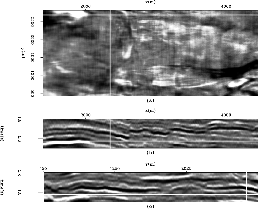
Figure ![[*]](http://sepwww.stanford.edu/latex2html/cross_ref_motif.gif) is an image of faulted Gulf of Mexico data. When a significant discontinuity occurs within a data-set, local dip estimators return incorrect estimates. Faults with significant displacement contaminate the dip estimation at the faults. This, in turn, results in unsatisfactory flattening results.
is an image of faulted Gulf of Mexico data. When a significant discontinuity occurs within a data-set, local dip estimators return incorrect estimates. Faults with significant displacement contaminate the dip estimation at the faults. This, in turn, results in unsatisfactory flattening results.
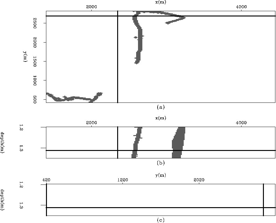
We use the crude binary weight cube shown in Figure ![[*]](http://sepwww.stanford.edu/latex2html/cross_ref_motif.gif) to identify areas where the inversion should ignore incorrect dips. This weight was created by manual picking. It should be noted that a suitable weight can also, in principle, be made from an automatic fault detector.
to identify areas where the inversion should ignore incorrect dips. This weight was created by manual picking. It should be noted that a suitable weight can also, in principle, be made from an automatic fault detector.
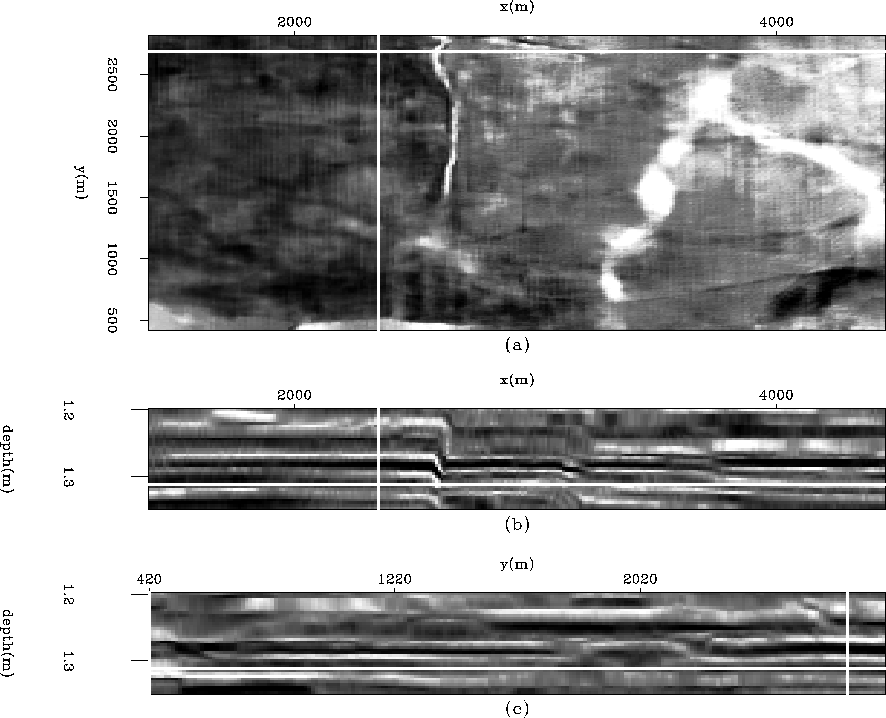
The flattening results are shown in Figure ![[*]](http://sepwww.stanford.edu/latex2html/cross_ref_motif.gif) . Notice that the horizons are flat, even directly across from the fault. Also, notice the presence of a channel in the horizon slice. Figure
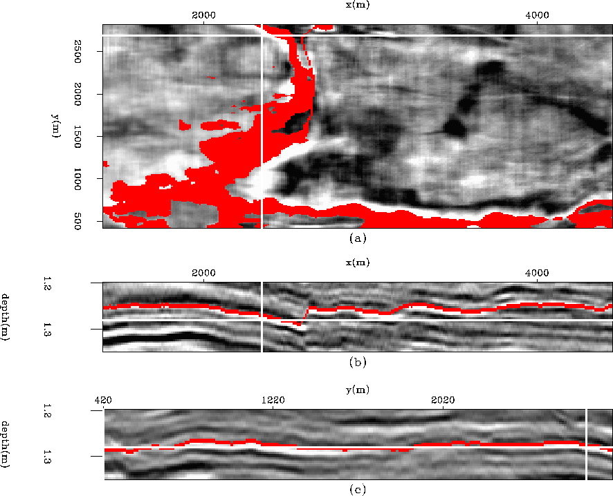
. Notice that the horizons are flat, even directly across from the fault. Also, notice the presence of a channel in the horizon slice. Figure ![[*]](http://sepwww.stanford.edu/latex2html/cross_ref_motif.gif) shows the original data with one unflattened horizon overlying it. It successfully tracks the horizon even across the fault. The time slice at the top of Figure
shows the original data with one unflattened horizon overlying it. It successfully tracks the horizon even across the fault. The time slice at the top of Figure ![[*]](http://sepwww.stanford.edu/latex2html/cross_ref_motif.gif) shows a horizon that is being partially cut by the fault at about x=
shows a horizon that is being partially cut by the fault at about x= .
.
shoal
Figure 10 Faulted Chevron Gulf of Mexico data. The 2D vertical section shows fault with significant displacement (enough to cause our dip estimator to return erroneous values). (a) The time slice at time= . (b) An in-line section at y=
 . (c) A cross-line section at x=
 .
.


 shoal.wt
Figure 11 A weight identifying the faults data displayed in ![[*]](http://sepwww.stanford.edu/latex2html/cross_ref_motif.gif) . (a) The time slice at time=
. (a) The time slice at time= . (b) An in-line section at y=
 . (c) A cross-line section at x=
 .
.


 shoal.flat
Figure 12 The result of flattening of Figure ![[*]](http://sepwww.stanford.edu/latex2html/cross_ref_motif.gif) . (a) The horizon slice at time=
. (a) The horizon slice at time= . (b) An in-line section at y=
 . (c) A cross-line section at x=
 .
.


 shoal.horizon_overlay
Figure 13 The result of overlaying a tracked horizon on the image in Figure ![[*]](http://sepwww.stanford.edu/latex2html/cross_ref_motif.gif) . (a) The time slice at time=
. (a) The time slice at time= . (b) An in-line section at y=
 . (c) A cross-line section at x=
 .
.


Next: Discussion
Up: examples of 3D flattening
Previous: Elf North Sea Unconformity
Stanford Exploration Project
5/3/2005
![[*]](http://sepwww.stanford.edu/latex2html/cross_ref_motif.gif) to identify areas where the inversion should ignore incorrect dips. This weight was created by manual picking. It should be noted that a suitable weight can also, in principle, be made from an automatic fault detector.
to identify areas where the inversion should ignore incorrect dips. This weight was created by manual picking. It should be noted that a suitable weight can also, in principle, be made from an automatic fault detector.
![[*]](http://sepwww.stanford.edu/latex2html/cross_ref_motif.gif) is an image of faulted Gulf of Mexico data. When a significant discontinuity occurs within a data-set, local dip estimators return incorrect estimates. Faults with significant displacement contaminate the dip estimation at the faults. This, in turn, results in unsatisfactory flattening results.
is an image of faulted Gulf of Mexico data. When a significant discontinuity occurs within a data-set, local dip estimators return incorrect estimates. Faults with significant displacement contaminate the dip estimation at the faults. This, in turn, results in unsatisfactory flattening results.
![[*]](http://sepwww.stanford.edu/latex2html/cross_ref_motif.gif) to identify areas where the inversion should ignore incorrect dips. This weight was created by manual picking. It should be noted that a suitable weight can also, in principle, be made from an automatic fault detector.
to identify areas where the inversion should ignore incorrect dips. This weight was created by manual picking. It should be noted that a suitable weight can also, in principle, be made from an automatic fault detector.
![[*]](http://sepwww.stanford.edu/latex2html/cross_ref_motif.gif) . Notice that the horizons are flat, even directly across from the fault. Also, notice the presence of a channel in the horizon slice. Figure
. Notice that the horizons are flat, even directly across from the fault. Also, notice the presence of a channel in the horizon slice. Figure ![[*]](http://sepwww.stanford.edu/latex2html/cross_ref_motif.gif) shows the original data with one unflattened horizon overlying it. It successfully tracks the horizon even across the fault. The time slice at the top of Figure
shows the original data with one unflattened horizon overlying it. It successfully tracks the horizon even across the fault. The time slice at the top of Figure ![[*]](http://sepwww.stanford.edu/latex2html/cross_ref_motif.gif) shows a horizon that is being partially cut by the fault at about x=
shows a horizon that is being partially cut by the fault at about x=![]() .
.

![[*]](http://sepwww.stanford.edu/latex2html/cross_ref_motif.gif) . (a) The time slice at time=
. (a) The time slice at time=
![[*]](http://sepwww.stanford.edu/latex2html/cross_ref_motif.gif) . (a) The horizon slice at time=
. (a) The horizon slice at time=
![[*]](http://sepwww.stanford.edu/latex2html/cross_ref_motif.gif) . (a) The time slice at time=
. (a) The time slice at time=