Water-bottom multiple in Image Space

Given the kinematic equivalence between the water-bottom multiple and a primary from a reflector dipping at twice the dip angle, we can express the image space coordinates of the water-bottom multiple in terms of the data space coordinates by solving the system of equations presented by Fomel and Prucha 1999:

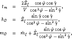$$\begin{eqnarray} t_m&=&\frac{2\hat{Z}_\xi}{V}\frac{\cos\hat{\varphi}\cos\hat{\ga... ...varphi}\cos\hat{\varphi}}{\cos^2\hat{\varphi}-\sin^2\hat{\gamma}},\end{eqnarray}$$ (13) (14) (15)

where $(\hat{X}_\xi,\hat{m}_\xi,\hat{\gamma})$ are the image space coordinates of the primary that is kinematically equivalent to the first order water-bottom multiple as mentioned n the previous section and $\hat{\varphi}=2\varphi$. The formal solution of these equations, for the image space coordinates is:

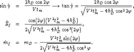$$\begin{eqnarray} \sin\hat{\gamma}&=&\frac{2h_D\cos 2\varphi}{Vt_m}\longrightarro... ...rac{V^2t_m^2\sin(2\varphi)}{2\sqrt{V^2t_m^2-4h_D^2\cos^2\varphi}}.\end{eqnarray}$$ (16) (17) (18)

These equations allow the computation of the impulse response of the water-bottom multiples in image space as a function of the aperture angle. More importantly, they are the starting point for understanding the kinematics of the data in 3D ADCIGs Tisserant and Biondi (2004), still a subject of research.