Start by binning the velocities in small bins, for example at 10 m/s (which would imply a maximum velocity error of 5 m/s, well below the likely error in the estimation of the velocities themselves) such that the vertical wavenumber kzl (that is, the dispersion relation), needs to be computed only a few hundred times and can thus be stored as a function of the horizontal wavenumber and the velocity. From the standpoint of the theoretical algorithm, all that changes is the selection process to choose the trace from the extrapolated wavefield that corresponds to the binned velocity at each spatial location. That is, instead of the selection being simply a multiplication by a Kronecker delta to choose l=j as it was before, it is now a multiplication with a Kronecker delta, to select l=p(j), that is, the wavefield that was migrated with the binned velocity corresponding to the bin of V(j). Equation (2) can then be rewritten as:
![]()
| |
(6) |
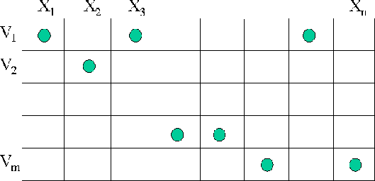
![[*]](http://sepwww.stanford.edu/latex2html/cross_ref_motif.gif) shows the velocity selection. This time, since
we don't have a wavefield migrated with each velocity, at each spatial
location, it is likely that several locations correspond to the same wavefield,
since they correspond to the same velocity bin. There is, obviously, just
one possible velocity at each spatial location, but many spatial locations
may share the same velocity. Also, it is possible for a particular velocity
not to be required at a specific depth step.
shows the velocity selection. This time, since
we don't have a wavefield migrated with each velocity, at each spatial
location, it is likely that several locations correspond to the same wavefield,
since they correspond to the same velocity bin. There is, obviously, just
one possible velocity at each spatial location, but many spatial locations
may share the same velocity. Also, it is possible for a particular velocity
not to be required at a specific depth step.
|
bin_vels2
Figure 2 Diagram illustrating velocity selection when there are fewer velocities than spatial locations. |  |