Radon domain

Figure through contain the inverted model domains associated with the four techniques explored herein. Clearly the sparsity of the results decrease toward the right. Direct interpretation of the model domain would be easier and more accurate with the BC, Cauchy, and l₁ results. Distict trains of energy in the hyperbolic and linear domains are visible. Without the clip set so low, the l₂ result is not as bad as these panels make it seem. A distinct fairway of energy, marginally larger than that presented in the l₁ result is visible. Velocity analysis of the gathers would likely be more accurate with the results that impose sparsity, especially at late times.

 

m.08
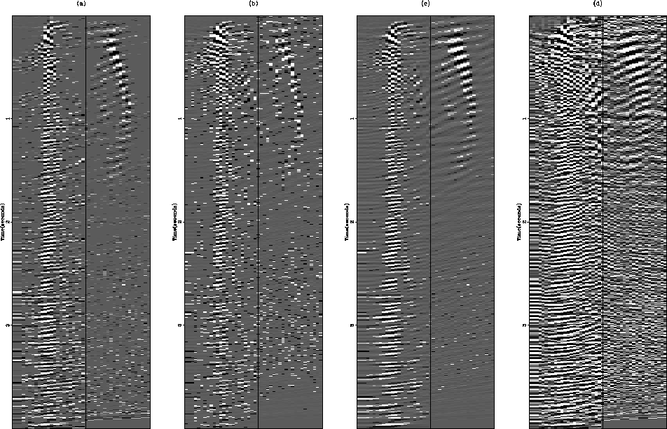
Figure 4 Model-space inversions of shot-gather 08 (Panel (a) from Figure ). The first half of the panels is HRT space and the second half is LRT space. Panel (a) shows the BC, Panel (b) the Cauchy, Panel (c) the l₁, and Panel (d) the l₂ inverted model spaces.

 

m.14
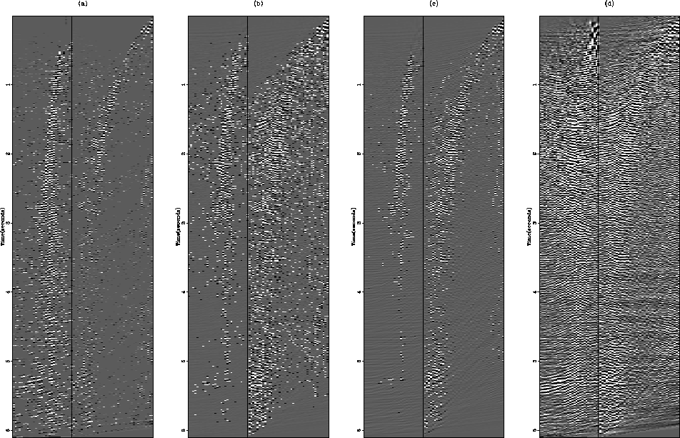
Figure 5 Model-space inversions of shot-gather 14 (Panel (b) from Figure ). The first half of the panels is HRT space and the second half is LRT space. Panel (a) shows the BC, Panel (b) the Cauchy, Panel (c) the l₁, and Panel (d) the l₂ inverted model spaces.

 

m.25r
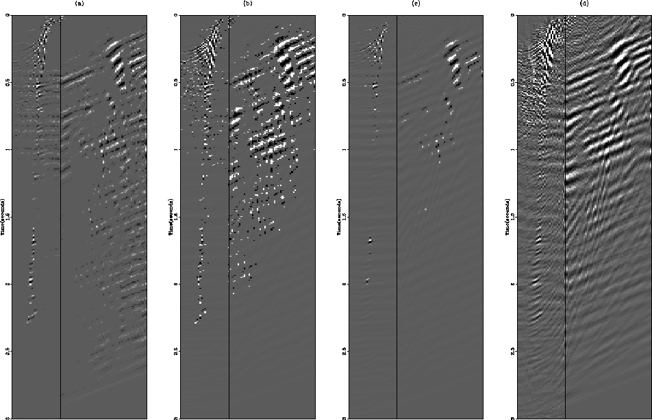
Figure 6 Model-space inversions of shot-gather 25 (Panel (c) from Figure ). The first half of the panels is HRT space and the second half is LRT space. Panel (a) shows the BC, Panel (b) the Cauchy, Panel (c) the l₁, and Panel (d) the l₂ inverted model spaces.

In general the l₁ inversion produced consistantly better model space realizations. While the differences are often minor, the method provides consistant, stable, high quality results.