Application to Herringbone data

The methods described above were applied to the herringbone synthetic. The fully-sampled data as well as the data with the hole are shown in Figure .

 

herr-orig
Figure 1 The herringbone data, (a) original data, and (b) data with hole.

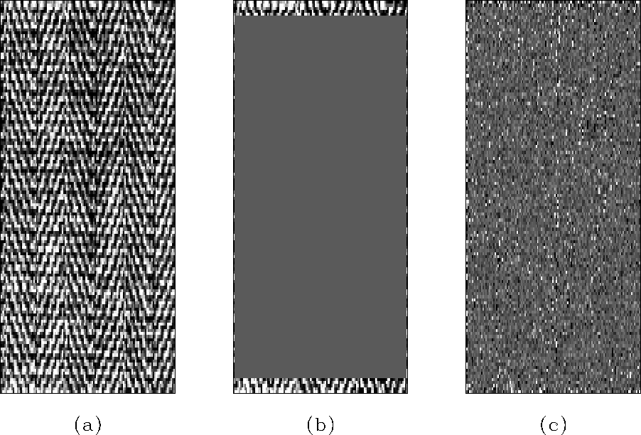
As a starting point, the hole was interpolated using a stationary PEF that was $9 \times 4$ coefficients, shown in Figure a. We can see how well the PEF has characterized the data by convolving the PEF with either the original data or the interpolated result. The result of convolving the PEF with the interpolated result is shown in Figure b. As has been previously noted, the PEF appears to miss the spines of the herringbone pattern, but gets the two slopes relatively well. When examining the result of random noise divided by that same stationary PEF (shown in Figure c) we can see the problem with the assumption of stationarity in that the two slopes present in the herringbone pattern are co-located throughout the simulation.

 

herr-stat
Figure 2 Stationary PEF result, (a) interpolated data, (b) interpolated data convolved with PEF, and (c) random noise divided by PEF.

The problems with co-located dips due to the assumption of stationarity can be avoided by using a non-stationary PEF. A $9 \times 2$ non-stationary PEF (with a total of about 16,000 filter coefficients) was estimated on the known data and then used to interpolate the missing data. As we can see from Figure a, the result is nearly perfect, which shouldn't be surprising given that the non-stationary PEF was estimated on the answer. Still, the restored version appears to have little of the problems of the interpolation smoothly decaying to zeros that was present in the stationary case. When convolving the PEF with the full dataset, we can see from the relative strength of the edge effects (in Figure b) that the filter perfectly captured the data. When we remove the edge effects, we see no trace of the spine of the herringbone, and the result looks very random as seen in Figure c.

 

herr-ns-known
Figure 3 Non-stationary PEF results, where the PEF is estimated on the complete data. (a) interpolated result. (b) PEF convolved with original data. (c) PEF convolved with original data with edge effects removed, and the result scaled.

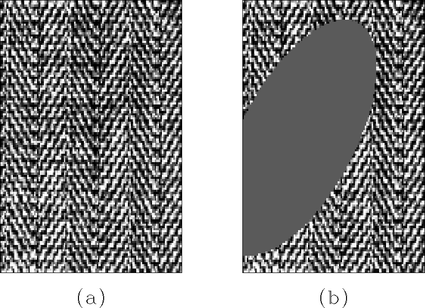
The previous test was a demonstration of the effectiveness of a non-stationary PEF as a container for information, but we had the answer before attempting to solve the problem. Next, we must resolve the issue of non-stationary PEFs with holes in them, which happens when we do not have the answer.

 

herr-ns-unknown
Figure 4 Non-stationary PEF results, where the PEF is estimated on the data with the hole. (a) The interpolation result using a filter with a hole in it. (b) non-stationary PEF convolved with original data. (c) non-stationary PEF convolved with interpolated result. (d) PEF from full data convolved with data with hole. (e) and (f): sections from a single filter lag for the model residual of fitting goal 5

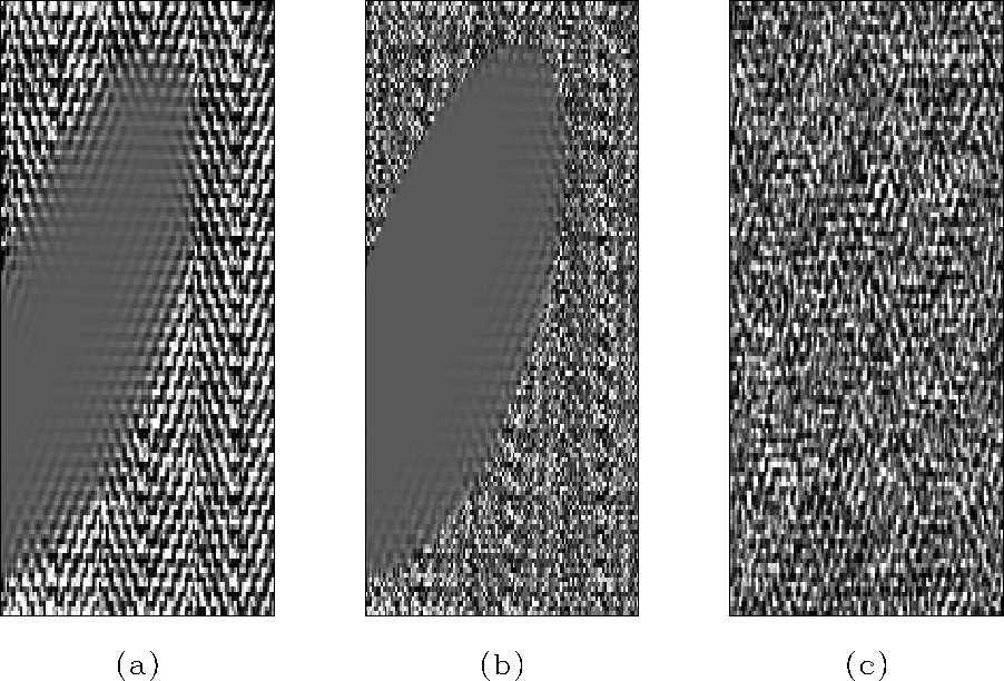
A more realistic starting point would be to estimate a PEF on the data with the hole and hope that the regularization term in fitting goal (5) would act as a method of interpolating the PEF in areas with missing data. As we can see from the results in Figure , this is clearly not the case. The restored data using a stationary PEF extends much further into the gap than the non-stationary PEF does. If we look at the model residual from fitting goal (5) shown in Figures e and f, we can start to see why. This is a portion of the model residual for two non-stationary filter coefficients over the entire space of the non-stationary PEF. We can see that as we move within the gap that the residual drops to zero, as the filter coefficients are also zero within this area. Relying upon the filter regularization to fill in gaps in the non-stationary filter does not put filters in holes.

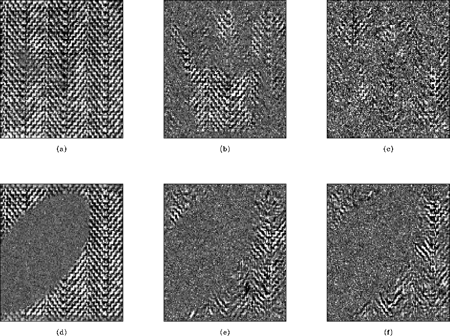
We can also look at the performance of the PEFs by looking at the random realizations as well as random noise divided by the non-stationary PEF, both shown in Figure . These results mostly confirm what we already know from Figure , however it is surprising to see that Figures b and c, which use the full data, are not as consistent as expected. The areas which contain the herringbone pattern are non consistent from simulation to simulation. This is not the case with the stationary PEF result of Figure c.

 

herr-realiz
Figure 5 (a) random realization of interpolation, (b) and (c) two sets of random numbers deconvolved with the PEF estimated on the complete data. (d) to (f): same as (a) to (c), except for a PEF estimated on the data with the hole.

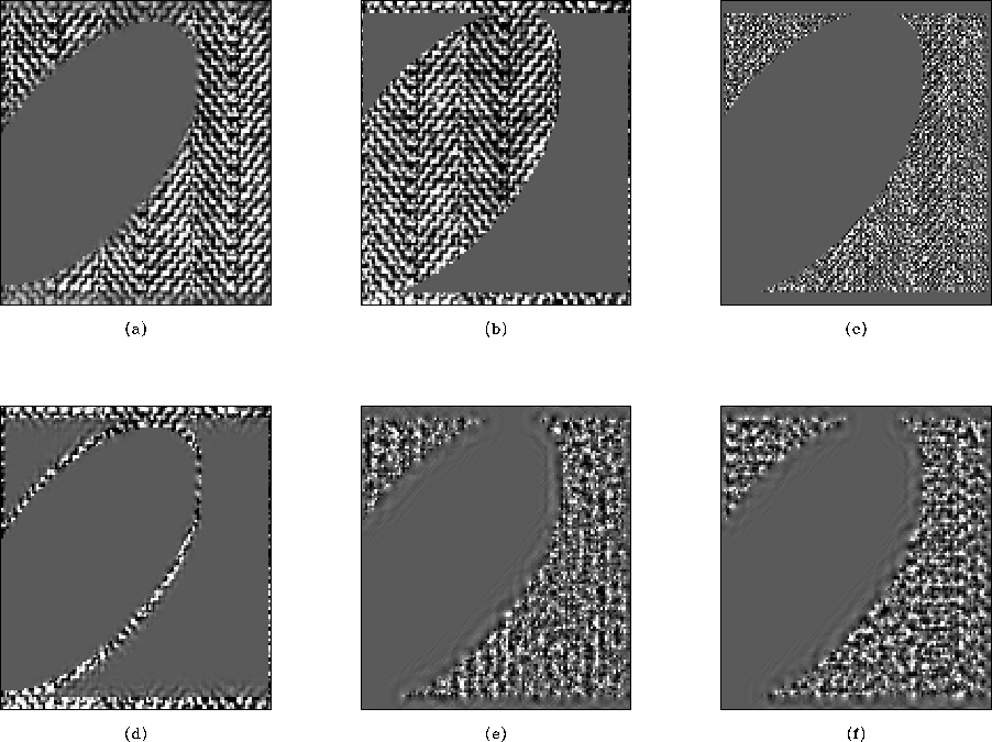
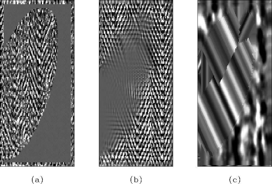
Instead of interpolating filter coefficients by relying on an isotropic roughener for regularization, a much simpler approach is taken. After the non-stationary PEF is estimated, the filter coefficients in areas with missing data are simply interpolated in a nearest-neighbor fashion with the nearest filter coefficients that are constrained by data. The results of using this method are shown in Figure . On the first panel (a), we can see that the signal that we want to destroy with our filter is partially gone, and the output looks much more random than before. On the second panel (b), we see that the interpolated result is better than any of the previous attempts. While there is only a single dip in any location, these dips are not in the correct locations as they do not follow the vertical spine of the herringbone. On the third panel (c), a single filter lag plotted with respect to space, we can clearly see the difference between filter coefficients that have been estimated on data, and those that have been interpolated from neighboring area with data.

 

herr-better
Figure 6 Results for PEF estimation with isotropic regularization and an isotropic nearest-neighbor search. (a) Convolution of the PEF with the fully-sampled data. (b) Interpolation with the PEF. We can see that the dips are no longer co-located, but do not match the spine of the herringbone pattern. (c) Filter coefficients from a single filter lag. We can see the isotropic smoothing of the filter coefficients as well as nearest neighbor smearing.

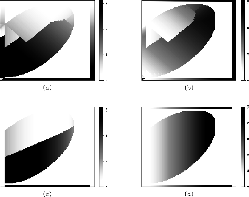
If we examine the mappings between the areas with no data and their nearest neighbors as shown in Figures a and b, we can see that the mappings do not correspond to the vertical trend present in the herringbone data. If we alter the nearest-neighbor interpolation so that no points outside of the vertical direction are considered, with the result shown in Figures c and d.

 

near
Figure 7 Nearest-neighbor coordinates of closest filters. (a) and (b): y and x locations (respectively) of nearest neighbors for missing data with an isotropic search. (c) and (d), the same, but when searching only vertically.

In addition to changing the filter interpolation so that it acts in a preferential direction, the regularization of the filter has been changed from an isotropic Laplacian to a derivative in the vertical direction. The results of using both of these new methods is shown in Figure . The first panel (a) shows how the missing signal is better attenuated with this method. The second panel (b) is the interpolation result, which is far superior to any other method shown in this paper. The correct dips are present in the correct locations. The amplitude of the interpolated result is not as uniform as would be desired, however. Finally, in the third panel (c), we can see that the interpolated filter coefficients are much more difficult to identify than with the previous method. The only obvious artifact is the seam caused by the nearest-neighbor interpolation when the interpolated data switched from one side of the gap to the other.

 

herr-best
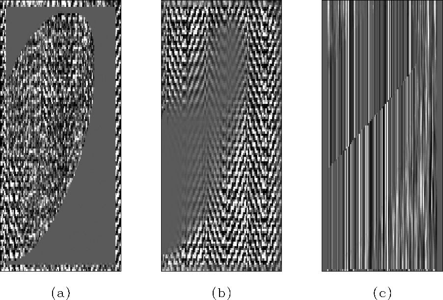Figure 8 Results for PEF estimation with a vertical derivative for regularization and a vertical nearest-neighbor search for missing coefficients. (a) Convolution of the PEF with the fully-sampled data. We can see that the result is more white than in Figure . (b) Interpolation with the PEF. Again, the result is better than in Figure . The dips are all in the correct locations, but the amplitude is not as high as it should be. (c) Filter coefficients from a single filter lag. The nearest-neighbor interpolated filter coefficients are now much harder to distinguish from the area where the PEF is estimated from local data.