![[*]](http://sepwww.stanford.edu/latex2html/cross_ref_motif.gif) ). Again, we assumed a land acquisition geometry, where the shots and receivers were positioned every
). Again, we assumed a land acquisition geometry, where the shots and receivers were positioned every
We created a synthetic dataset, using equation 6, from a model with a constant-reflectivity flat reflector lying beneath a Gaussian low velocity anomaly (Figure ![[*]](http://sepwww.stanford.edu/latex2html/cross_ref_motif.gif) ). Again, we assumed a land acquisition geometry, where the shots and receivers were positioned every
). Again, we assumed a land acquisition geometry, where the shots and receivers were positioned every ![]() on the interval
on the interval ![]() .
.
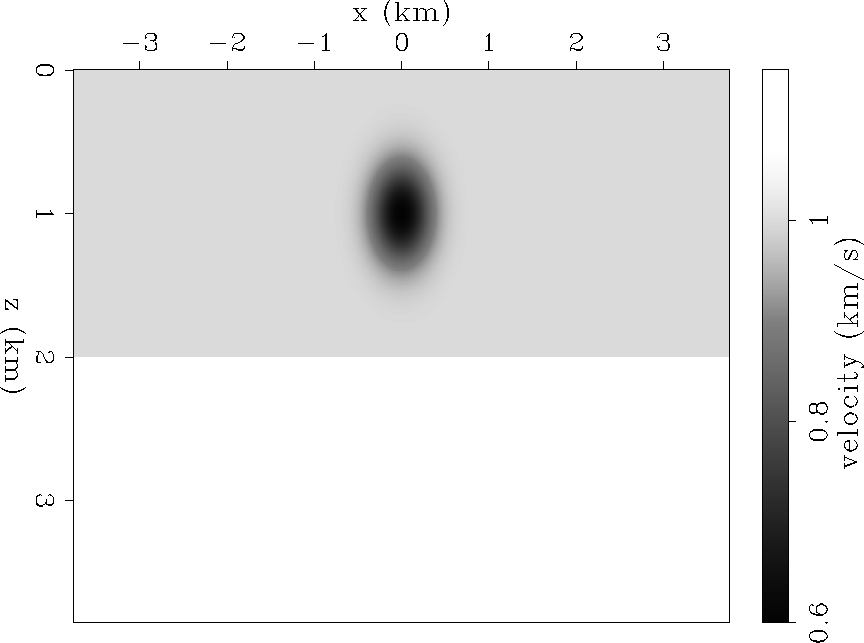 |
Figure ![[*]](http://sepwww.stanford.edu/latex2html/cross_ref_motif.gif) shows a
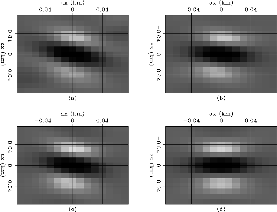
shows a ![]() coefficient filter at constant depth as the x coordinate moves from the corner to the center of the acquisition. Figure
coefficient filter at constant depth as the x coordinate moves from the corner to the center of the acquisition. Figure ![[*]](http://sepwww.stanford.edu/latex2html/cross_ref_motif.gif) a shows point 1, with coordinates
a shows point 1, with coordinates ![]() (corner of the acquisition). Figure
(corner of the acquisition). Figure ![[*]](http://sepwww.stanford.edu/latex2html/cross_ref_motif.gif) b shows point 2, with coordinates
b shows point 2, with coordinates ![]() . Figure
. Figure ![[*]](http://sepwww.stanford.edu/latex2html/cross_ref_motif.gif) c shows point 3, with coordinates
c shows point 3, with coordinates ![]() . Figure
. Figure ![[*]](http://sepwww.stanford.edu/latex2html/cross_ref_motif.gif) d shows point 4, with coordinates
d shows point 4, with coordinates ![]() (at the center of the acquisition).
Figure
(at the center of the acquisition).
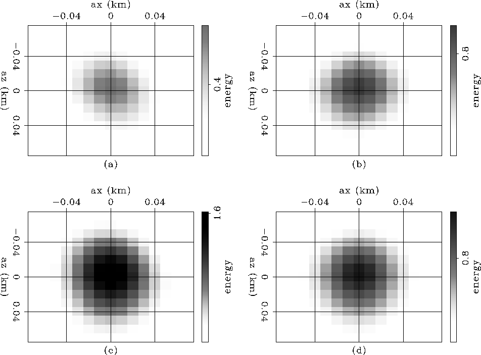
Figure ![[*]](http://sepwww.stanford.edu/latex2html/cross_ref_motif.gif) shows the envelope of the
shows the envelope of the ![]() coefficient filter shown in Figure
coefficient filter shown in Figure ![[*]](http://sepwww.stanford.edu/latex2html/cross_ref_motif.gif) . Differently to the constant velocity case, the higher energy is at point 3 (
. Differently to the constant velocity case, the higher energy is at point 3 (![]() ) (away from the center). This is due to a focusing effect created by the Gaussian velocity anomaly. To correct this effect we computed the least-squares inverse image, by the method described in the above section.
) (away from the center). This is due to a focusing effect created by the Gaussian velocity anomaly. To correct this effect we computed the least-squares inverse image, by the method described in the above section.
 |
 |
As with the previous example, two different numbers of filter coefficients were used. Figures ![[*]](http://sepwww.stanford.edu/latex2html/cross_ref_motif.gif) and
and ![[*]](http://sepwww.stanford.edu/latex2html/cross_ref_motif.gif) show the inversion results for a filter of
show the inversion results for a filter of ![]() coefficients, whereas Figures
coefficients, whereas Figures ![[*]](http://sepwww.stanford.edu/latex2html/cross_ref_motif.gif) and
and ![[*]](http://sepwww.stanford.edu/latex2html/cross_ref_motif.gif) show the inversion results for a filter of
show the inversion results for a filter of ![]() coefficients. Figure
coefficients. Figure ![[*]](http://sepwww.stanford.edu/latex2html/cross_ref_motif.gif) shows a comparison of the best results of both filter sizes.
shows a comparison of the best results of both filter sizes.
The panels in Figure ![[*]](http://sepwww.stanford.edu/latex2html/cross_ref_motif.gif) show the least-squares inverse image for different number of iterations for a filter of
show the least-squares inverse image for different number of iterations for a filter of ![]() coefficients:
coefficients: ![[*]](http://sepwww.stanford.edu/latex2html/cross_ref_motif.gif) a for 10 iterations,
a for 10 iterations, ![[*]](http://sepwww.stanford.edu/latex2html/cross_ref_motif.gif) b for 20 iterations,
b for 20 iterations, ![[*]](http://sepwww.stanford.edu/latex2html/cross_ref_motif.gif) c for 100 iterations, and
c for 100 iterations, and ![[*]](http://sepwww.stanford.edu/latex2html/cross_ref_motif.gif) d for migration. Notice how the image amplitudes become more even, but as the number of iterations increase the result becomes unstable.
Figure
d for migration. Notice how the image amplitudes become more even, but as the number of iterations increase the result becomes unstable.
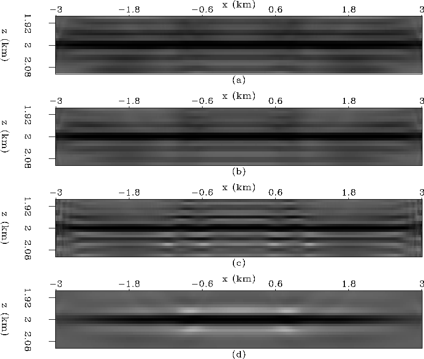
Figure ![[*]](http://sepwww.stanford.edu/latex2html/cross_ref_motif.gif) compares the same least-squares inverse image results at the reflector depth. The image amplitude after 10 iterations is the best result. The conjugate gradient algorithm further balances the image amplitudes, which reduces the effects of acquisition geometry and the bandlimited characteristic of the seismic data. But is not as good reducing the focusing effect (amplitude anomaly at
compares the same least-squares inverse image results at the reflector depth. The image amplitude after 10 iterations is the best result. The conjugate gradient algorithm further balances the image amplitudes, which reduces the effects of acquisition geometry and the bandlimited characteristic of the seismic data. But is not as good reducing the focusing effect (amplitude anomaly at ![]() ).
).
 |
|
inv_pp_11
Figure 12 Amplitudes extracted at reflector depth from Figure ![[*]](http://sepwww.stanford.edu/latex2html/cross_ref_motif.gif) , filter size of , filter size of | 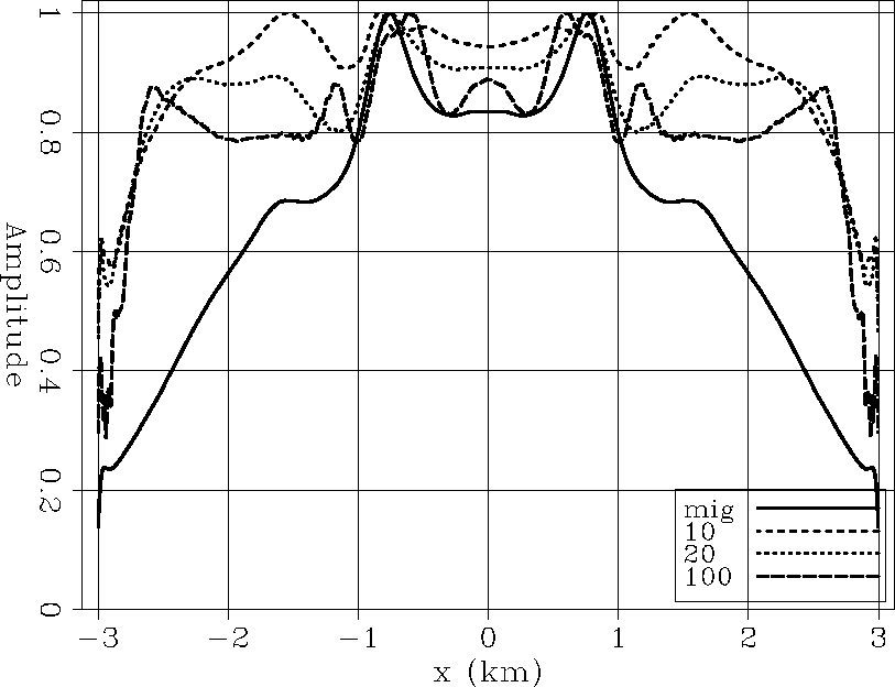 |
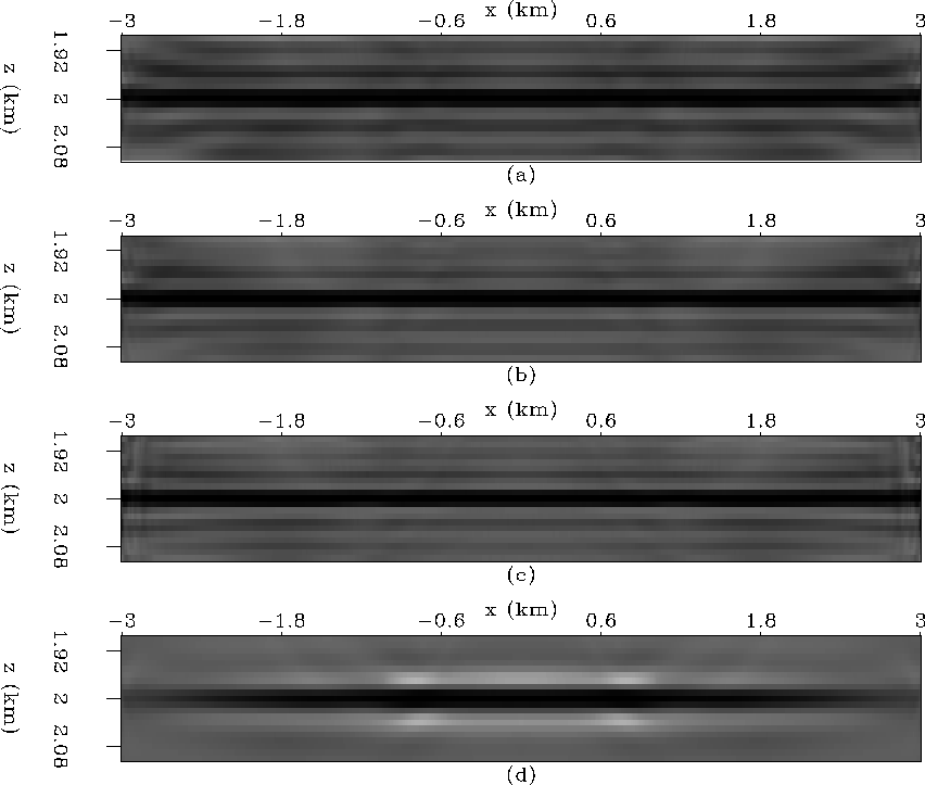
The panels in Figure ![[*]](http://sepwww.stanford.edu/latex2html/cross_ref_motif.gif) show the least-squares inverse image for different number of iterations for a filter of
show the least-squares inverse image for different number of iterations for a filter of ![]() coefficients:
coefficients: ![[*]](http://sepwww.stanford.edu/latex2html/cross_ref_motif.gif) a for 10 iterations,
a for 10 iterations, ![[*]](http://sepwww.stanford.edu/latex2html/cross_ref_motif.gif) b for 20 iterations,
b for 20 iterations, ![[*]](http://sepwww.stanford.edu/latex2html/cross_ref_motif.gif) c for 100 iterations, and
c for 100 iterations, and ![[*]](http://sepwww.stanford.edu/latex2html/cross_ref_motif.gif) d for migration. Notice how the image amplitudes become more even, as the number of iterations increase.
Figure
d for migration. Notice how the image amplitudes become more even, as the number of iterations increase.
Figure ![[*]](http://sepwww.stanford.edu/latex2html/cross_ref_motif.gif) shows the comparison of the same least-squares inverse image results at the reflector depth. The image amplitude after 100 iterations is the best result. The conjugate gradient algorithm further balances the image amplitudes, reducing the focusing effect as well as the effects of the acquisition geometry and the bandlimited characteristic of the seismic data.
shows the comparison of the same least-squares inverse image results at the reflector depth. The image amplitude after 100 iterations is the best result. The conjugate gradient algorithm further balances the image amplitudes, reducing the focusing effect as well as the effects of the acquisition geometry and the bandlimited characteristic of the seismic data.
 |
|
inv_pp_15
Figure 14 Amplitudes extracted at reflector depth from Figure ![[*]](http://sepwww.stanford.edu/latex2html/cross_ref_motif.gif) , filter size of , filter size of | 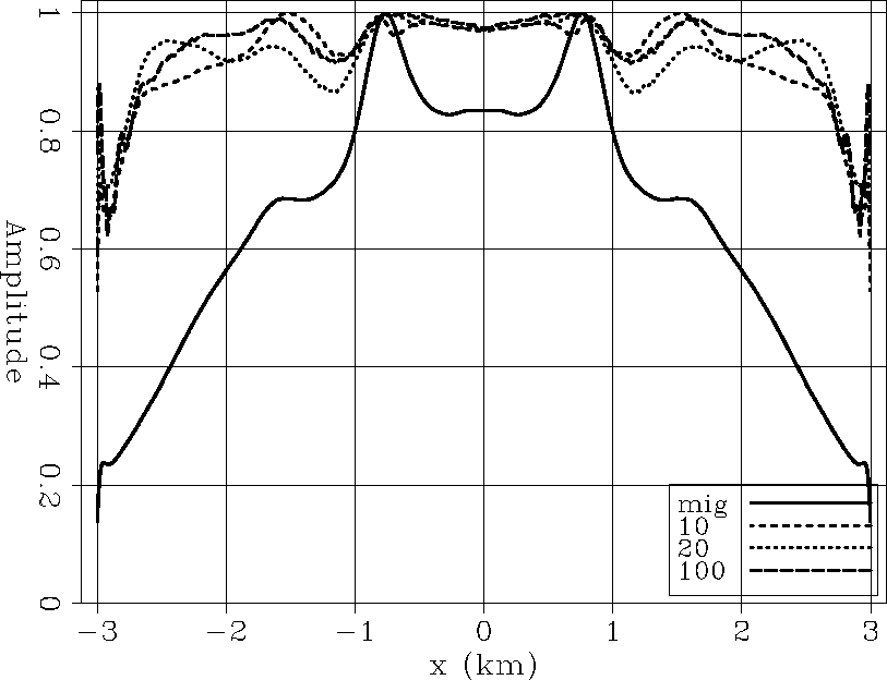 |
Figure ![[*]](http://sepwww.stanford.edu/latex2html/cross_ref_motif.gif) the migration result to the 100 iterations inversion results for filter sizes
the migration result to the 100 iterations inversion results for filter sizes ![]() coefficients,
coefficients, ![]() coefficients. There is a big difference in the recover amplitudes for the different filter sizes being the
coefficients. There is a big difference in the recover amplitudes for the different filter sizes being the ![]() coefficient filter the one that better reduces the effect of the focusing effect on the amplitudes. More research needs to be done to find a way to a priori predict the proper filter size.
coefficient filter the one that better reduces the effect of the focusing effect on the amplitudes. More research needs to be done to find a way to a priori predict the proper filter size.
|
inv_filter
Figure 15 Comparison the migration result to the 100 iterations inversion results for filter sizes | 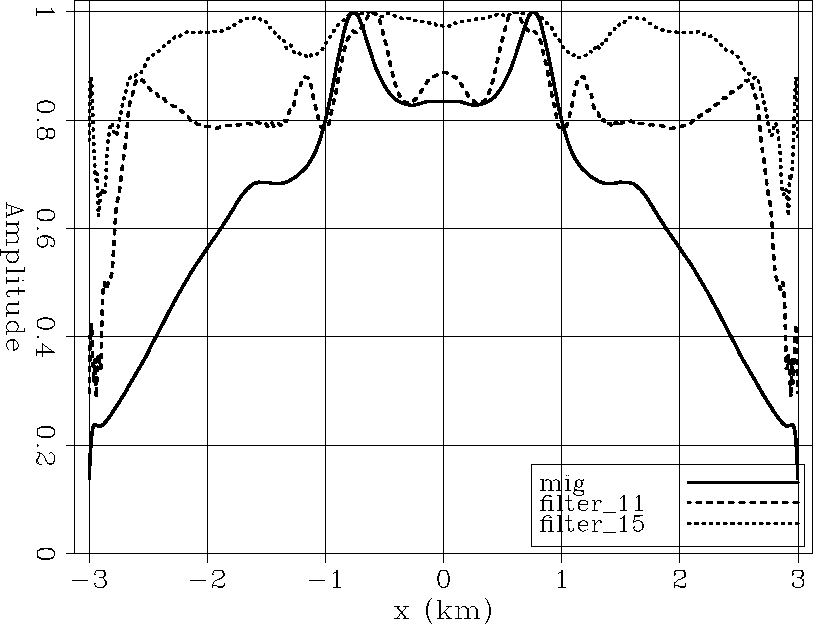 |