

Next: CONCLUSION
Up: R. Clapp: Velocity uncertainty
Previous: Multiple realization methodology
Clapp (2004) took nine different realizations of a single
linearizion of a complex synthetic model (Figure ![[*]](http://sepwww.stanford.edu/latex2html/cross_ref_motif.gif) ).
There were several problems with this approach.
The most significant problem was that a single non-linear iteration,
was far from sufficient. After one iteration, we still
have significant move-out that another non-linear
iteration of tomography has a chance of using.
When doing multiple non-linear iterations we have
two choices to make at each iteration.
First, should we use the minimum energy model (no random
perturbation) or introduce random perturbations?
Second, if we are adding random perturbations, how
many models should we create at each non-linear iteration?
model
).
There were several problems with this approach.
The most significant problem was that a single non-linear iteration,
was far from sufficient. After one iteration, we still
have significant move-out that another non-linear
iteration of tomography has a chance of using.
When doing multiple non-linear iterations we have
two choices to make at each iteration.
First, should we use the minimum energy model (no random
perturbation) or introduce random perturbations?
Second, if we are adding random perturbations, how
many models should we create at each non-linear iteration?
model
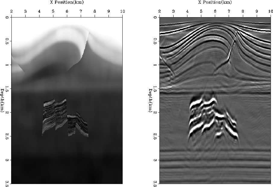
Figure 1 The left panels
shows the velocity model used as input to
the finite difference scheme used to create the
data.
The right panel is the resulting migrating the data with
the correct velocity. The fine structure seen below 1.6km is
the reservoir.
![[*]](http://sepwww.stanford.edu/latex2html/movie.gif)


For this experiment I decided to create five random
perturbed models in the first non-linear iteration.
From these five models I generated twenty five models
during the second non-linear iteration. I then used
these twenty-five models in a conventional migration
velocity updating scheme. This gives some measure
on the effect of the starting guess on the final solution.
Each of the twenty-five models were equally reasonable
points from which start a tomographic loop. The difference
between the final images gives me some measure of the
uncertainty in this updating scheme.
The left panel of Figure ![[*]](http://sepwww.stanford.edu/latex2html/cross_ref_motif.gif) shows
my starting guess for
the velocity problem. The right
panel shows the resulting image. The velocity was
created by applying a strong
smoother to the correct velocity field
then scaling the resulting model by .9.
Figure
shows
my starting guess for
the velocity problem. The right
panel shows the resulting image. The velocity was
created by applying a strong
smoother to the correct velocity field
then scaling the resulting model by .9.
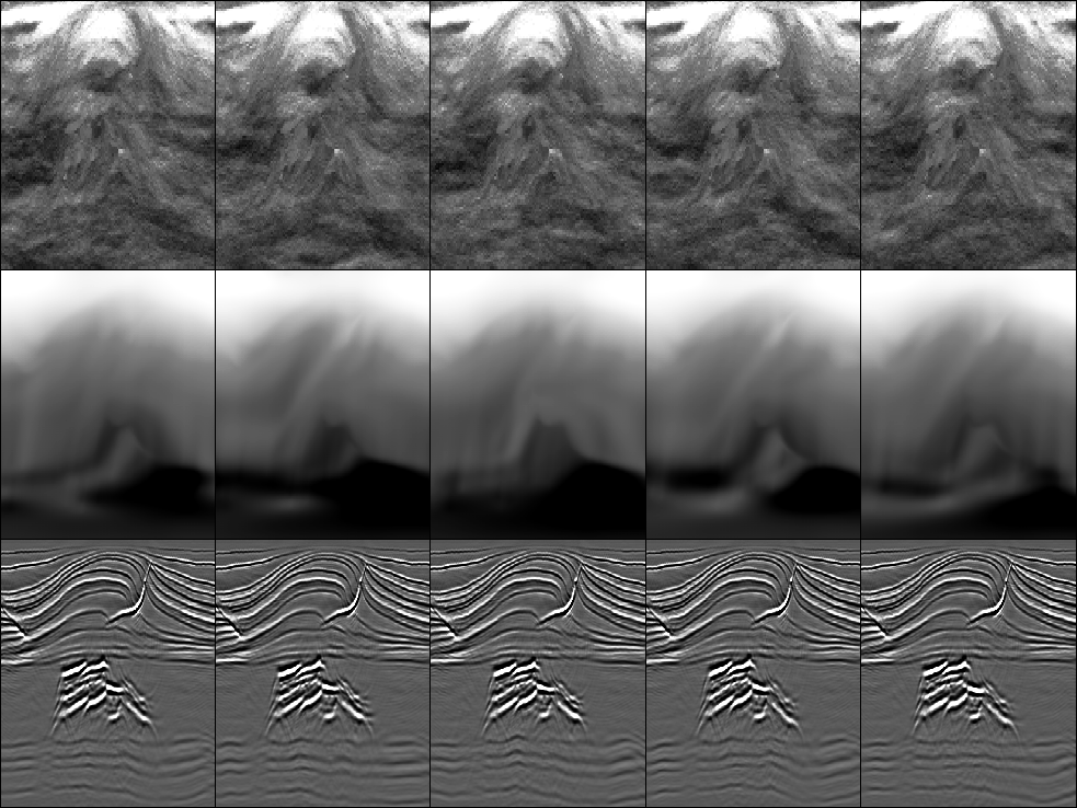
Figure ![[*]](http://sepwww.stanford.edu/latex2html/cross_ref_motif.gif) shows the results after
one non-linear iteration. The top panel are the five
realizations of
shows the results after
one non-linear iteration. The top panel are the five
realizations of  . The center panels
are the resulting five velocity models, and
the bottom five panels are the migrated images using
these velocity models. The anticline
trend is in all of the realizations but
we still see significant differences in how the velocity
estimate deals with the listric fault.
iter0
Figure 2 The left panel
shows the initial velocity model. The
right panel the resulting migration.
![[*]](http://sepwww.stanford.edu/latex2html/movie.gif)


 iter1
iter1
Figure 3 The top panel are the five
realizations of  . The center panels
are the resulting five velocity models, and
the bottom five panels are the migrated images using
these velocity models.
![[*]](http://sepwww.stanford.edu/latex2html/movie.gif)


After four iterations, now with twenty-five
different models, the differences are more dramatic.
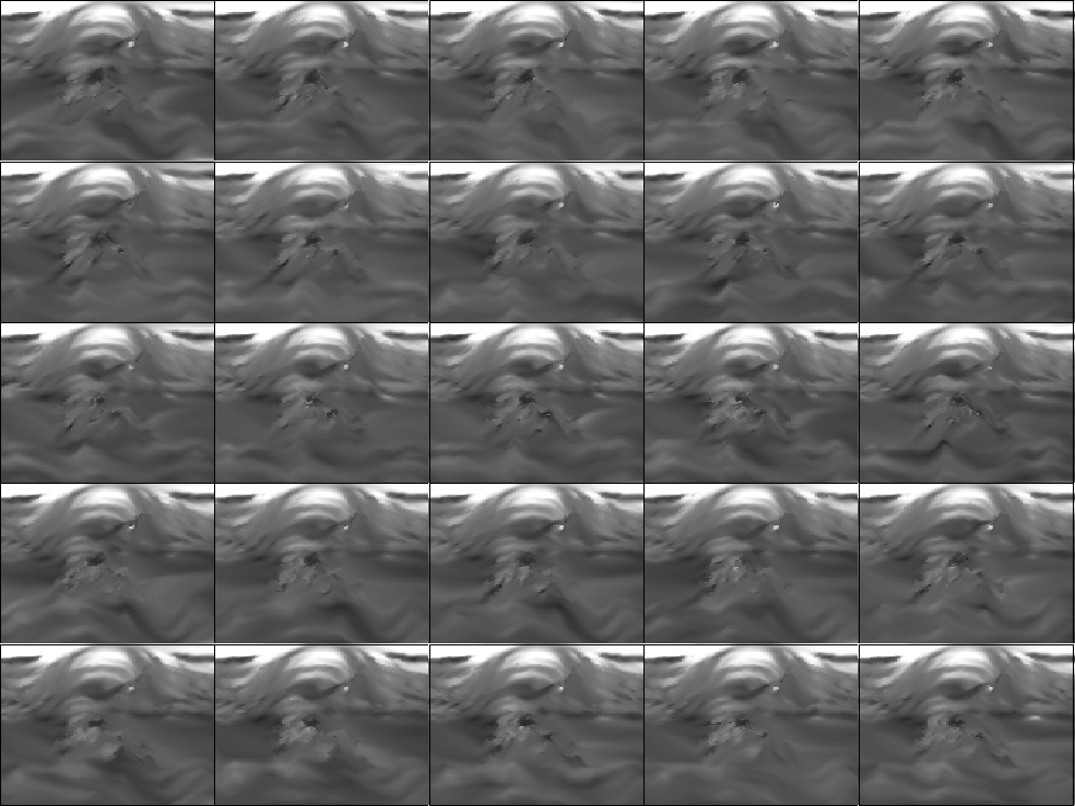
Figure ![[*]](http://sepwww.stanford.edu/latex2html/cross_ref_motif.gif) show the twenty-five different
gamma panels. We see an overall reduction in
the amount move-out (closer to gray), but the
realizations still have significantly
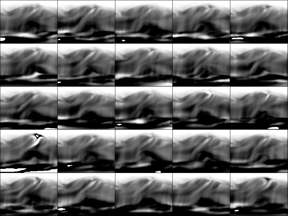
different character. The twenty-five velocity
models (Figure
show the twenty-five different
gamma panels. We see an overall reduction in
the amount move-out (closer to gray), but the
realizations still have significantly
different character. The twenty-five velocity
models (Figure ![[*]](http://sepwww.stanford.edu/latex2html/cross_ref_motif.gif) ) also show
significant variation, especially as we go deeper
in the model.
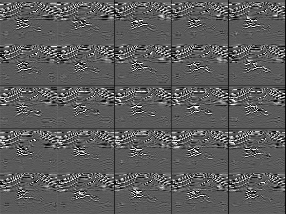
After four iterations we see significant differences
in the images (Figure
) also show
significant variation, especially as we go deeper
in the model.
After four iterations we see significant differences
in the images (Figure ![[*]](http://sepwww.stanford.edu/latex2html/cross_ref_motif.gif) ). In most of the models we
have focused the anticline structure, but the images have
significant variation below. The basement reflectors
are discontinuous in many of the models.
). In most of the models we
have focused the anticline structure, but the images have
significant variation below. The basement reflectors
are discontinuous in many of the models.
iter3_g
Figure 4 The twenty-five
gamma panels after the third non-linear iteration.
Note how we are overall closer to 1.0 (gray), but
we still see differences in the various panels.


 iter4_v
Figure 5 The final twenty-five
velocity models.
![[*]](http://sepwww.stanford.edu/latex2html/movie.gif)


 iter4_i
Figure 6 The twenty-five
different images. Note the differences, especially
in the reservoir.


Next: CONCLUSION
Up: R. Clapp: Velocity uncertainty
Previous: Multiple realization methodology
Stanford Exploration Project
10/23/2004
![[*]](http://sepwww.stanford.edu/latex2html/movie.gif)
![[*]](http://sepwww.stanford.edu/latex2html/cross_ref_motif.gif) ).
There were several problems with this approach.
The most significant problem was that a single non-linear iteration,
was far from sufficient. After one iteration, we still
have significant move-out that another non-linear
iteration of tomography has a chance of using.
When doing multiple non-linear iterations we have
two choices to make at each iteration.
First, should we use the minimum energy model (no random
perturbation) or introduce random perturbations?
Second, if we are adding random perturbations, how
many models should we create at each non-linear iteration?
).
There were several problems with this approach.
The most significant problem was that a single non-linear iteration,
was far from sufficient. After one iteration, we still
have significant move-out that another non-linear
iteration of tomography has a chance of using.
When doing multiple non-linear iterations we have
two choices to make at each iteration.
First, should we use the minimum energy model (no random
perturbation) or introduce random perturbations?
Second, if we are adding random perturbations, how
many models should we create at each non-linear iteration?

