|
inverse
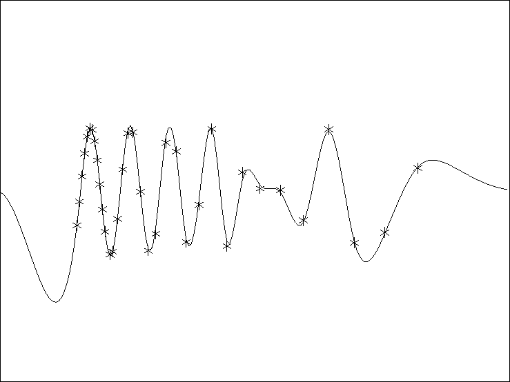
Figure 1 A simple linear interpolation result unsing the out-of-core library.The `*' are the known data and the line is the estimated curve. |  |
args=SEP.par.sep_args() #get arguments
dname=args.par("data",error=1)
mname=args.par("model",error=1)
We then create the data and model float vectors.
In the case of the data is read from a file
and the model is defined.
data =SEP.sep_vector.sfloat(tag=dname)
model=SEP.sep_vector.sfloat(name=mname)
model.set_axis(200,0.,.4)
We then write out the description of the model to disk and zero the file.
model.write_file()
model.zero()
Our data fitting operator is simple linear interpolation. It takes the coordinates of the data as input and we direct the stdout to /dev/null.
interp_args=SEP.par.sep_pars(name="interp")
interp_args.add_string("coord=coord.H")
interp_args.add_param(">","/dev/null")
We create the argument list for the preconditioner.
In this case we just need to direct stdout to /dev/null
and specify the type of filter.
precpar=SEP.par.sep_pars(name="devnull")
precpar.add_param("filter",2)0
precpar.add_param(">","/dev/null")0
Next we create our operator objects. In both cases the domain vector is the model. In the case of the interpolation operator the range is the data. For the preconditioning the range is also described by the model space.
interp=SEP.operator.oc("Interp1.x",model,data,pars=interp_args)
prec=SEP.operator.oc("prec.x",model,model,pars=precpar)
We create our step function.
step=SEP.cgstep.cgstep("matcg")
Finally we create our solver object and
iterate for 20 iterations. Figure ![[*]](http://sepwww.stanford.edu/latex2html/cross_ref_motif.gif) shows
the result of the inversion. The `*' are the known data
and the line is the estimated curve.
shows
the result of the inversion. The `*' are the known data
and the line is the estimated curve.
|
inverse
Figure 1 A simple linear interpolation result unsing the out-of-core library.The `*' are the known data and the line is the estimated curve. |  |
solver=SEP.solver.prec("interp1d",model,data,interp,prec,step,20,.1,verb=0)
if not solver.solve():
  SEP.util.err( "Trouble iterating")