


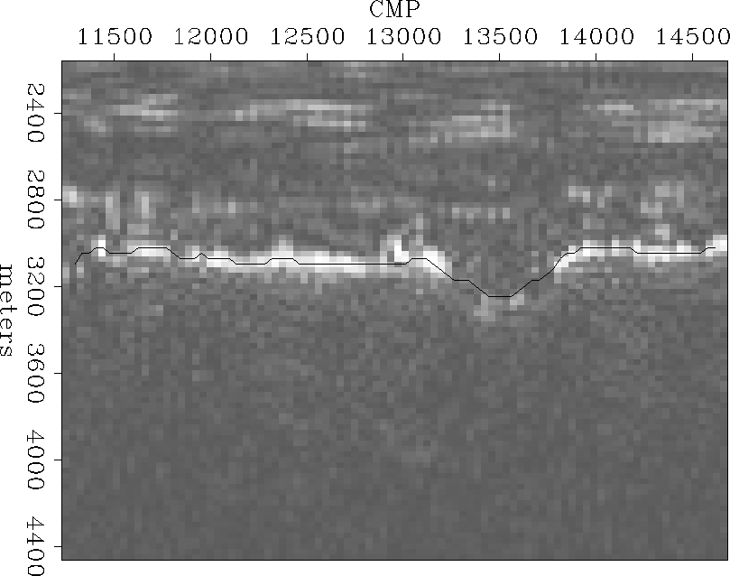
![[*]](http://sepwww.stanford.edu/latex2html/cross_ref_motif.gif) . The salt boundary is at approximately 3200 ms. The instantaneous amplitude is shown is Figure . Notice that it isn't too obvious where to pick the salt boundary near Cmp 13500.
. The salt boundary is at approximately 3200 ms. The instantaneous amplitude is shown is Figure . Notice that it isn't too obvious where to pick the salt boundary near Cmp 13500.
The resulting ![]() eigenvector is shown in Figure and a contour plot is shown in Figure . Notice that the contours are spread in areas where the amplitude of the salt boundary is low and the tracking is therefore less certain.
eigenvector is shown in Figure and a contour plot is shown in Figure . Notice that the contours are spread in areas where the amplitude of the salt boundary is low and the tracking is therefore less certain.
Lastly, Figure shows the instantaneous amplitude with the partition with the minimum normalized cut overlain. It tracks the salt boundary even across the challenging area around Cmp 13500.
 |


