Background

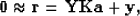
A prediction-error filter is estimated by solving a minimization problem where known data is convolved ($\bf{Y}$) with an unknown filter ($\bf{a}$), so  

$$\bold 0 \approx \bold r = \bf{Ya} ,$$ (1)

where the first coefficient of $\bf{a}$ is constrained to be unity. This can be written as  

$$\bold 0 \approx \bold r = \bf{YKa} + \bold y ,$$ (2)

where $\bf{K}$ is a mask for the first PEF coefficient, and $\bf{y}$ is simply a copy of the data. Writing out the matrices for a PEF with 3 coefficients and for 7 data samples looks like  

$$\bold 0 \quad \approx \quad \bold r = \left[ \begin{array} ... ... \\ y_3 \\ y_4 \\ y_5 \\ y_6 \end{array} \right] .$$ (3)

The previous equations have all been for a 1D case. By use of the helical coordinate Claerbout (1998), these equations can easily be extended to higher dimensions.

In the case of missing data, a diagonal weight ($\bf{W}$) can be introduced that is when a missing data point is in the equation, and 1 where all data are present. This weight can also be used to eliminate edge effects caused by helical convolution.

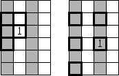
When data are interlaced, a PEF can be estimated by spacing filter coefficients during convolution, so that they fall on known data. An example of this filter spacing is shown in Figure . The problem with this methods is that the data must be regularly sampled in all dimensions.

 

interlace Figure 1 Examples of PEFs on interlaced data. White bins are empty, gray have data. Left: A PEF cannot be estimated due to too much missing data. Right: The spaced PEF can be estimated on interlaced data.