

Next: Selection Mechanism
Up: Parameter Selection
Previous: Model Parameter Encoding
Ideally, the population size should be large enough to guarantee adequate
genetic diversity yet small enough for efficient processing. In particular,
the number of cost-function evaluations is proportional to the population size.
Equation 1 corresponds to Goldberg's criterion Goldberg (1989b)
of increasing the population size exponentially with the increase in the
number of model parameters (assuming binary encoding).
|
npopsize=order[(l/k)(2**k)]
|
(1) |
In this equation, l is the number of bits in the chromosome and k the
order of the
schemata of interest (schemata is plural for schema ![[*]](http://sepwww.stanford.edu/latex2html/foot_motif.gif) ). This criterion, however, may result in populations too large
when the number of model parameters and so the length of the chromosome is
large. In this
case, for example, with 99 model parameters, each encoded with 10 bits,
even for a relatively low-order schema of 5 bits the population size would
have to be larger than 3000 individuals. Such large populations may require
many cost-function evaluations and a lot of memory. Most applications reported in
the literature use population sizes between 50 and 200 individuals and I am
unaware of any reported use of a population larger than 1000 individuals. For
the purpose of the present application I decided to try a relatively wide
number of population sizes using for the other evolution parameters
``reasonably'' standard choices. For example, I used uniform crossover with
a probability
of 0.6, jump mutation probability equal to 1/npopsize (large populations have
larger genetic diversity and so less need for jump mutation) and creep
mutation probability equal to the number of bits per model parameter times
the jump mutation rate. Also, for this first set of tests I allowed both niching
(sharing) and elitism of the best individual.
). This criterion, however, may result in populations too large
when the number of model parameters and so the length of the chromosome is
large. In this
case, for example, with 99 model parameters, each encoded with 10 bits,
even for a relatively low-order schema of 5 bits the population size would
have to be larger than 3000 individuals. Such large populations may require
many cost-function evaluations and a lot of memory. Most applications reported in
the literature use population sizes between 50 and 200 individuals and I am
unaware of any reported use of a population larger than 1000 individuals. For
the purpose of the present application I decided to try a relatively wide
number of population sizes using for the other evolution parameters
``reasonably'' standard choices. For example, I used uniform crossover with
a probability
of 0.6, jump mutation probability equal to 1/npopsize (large populations have
larger genetic diversity and so less need for jump mutation) and creep
mutation probability equal to the number of bits per model parameter times
the jump mutation rate. Also, for this first set of tests I allowed both niching
(sharing) and elitism of the best individual.
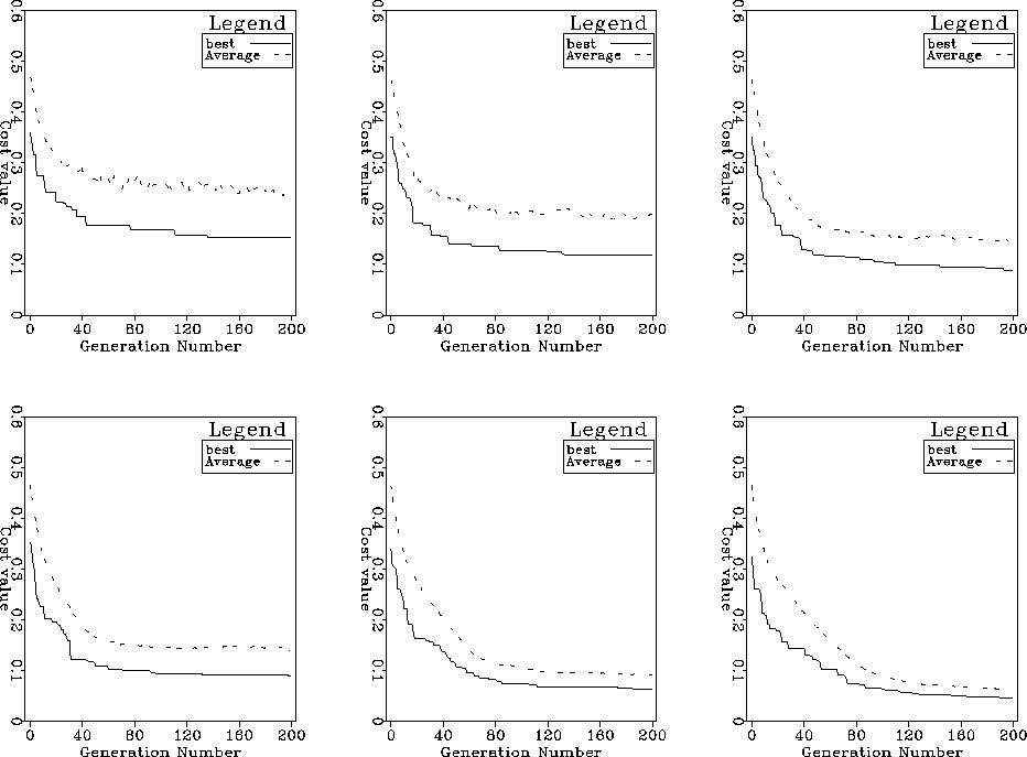
The top panels of Figure ![[*]](http://sepwww.stanford.edu/latex2html/cross_ref_motif.gif) , from left to right,
show a comparison of convergence rate as a function of number of generations
for population sizes of 50, 100, 200 individuals whereas the bottom panels
show similar curves for population sizes of 250, 500 and 1000 individuals.
As expected, the larger populations produce better convergence after a fixed
number of generations. This is not a fair test, however, since the number of
cost-function evaluations is proportional to the population size.
Figure
, from left to right,
show a comparison of convergence rate as a function of number of generations
for population sizes of 50, 100, 200 individuals whereas the bottom panels
show similar curves for population sizes of 250, 500 and 1000 individuals.
As expected, the larger populations produce better convergence after a fixed
number of generations. This is not a fair test, however, since the number of
cost-function evaluations is proportional to the population size.
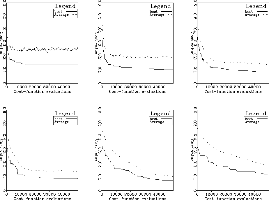
Figure ![[*]](http://sepwww.stanford.edu/latex2html/cross_ref_motif.gif) shows the same curves for a fixed
number of function evaluations. Clearly, there is a practical range of
optimum population sizes about 200 or 250 individuals.
For all the following tests I used a population of 200 individuals.
Figure
shows the same curves for a fixed
number of function evaluations. Clearly, there is a practical range of
optimum population sizes about 200 or 250 individuals.
For all the following tests I used a population of 200 individuals.
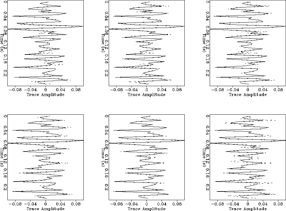
Figure ![[*]](http://sepwww.stanford.edu/latex2html/cross_ref_motif.gif) shows a comparison of the reference
trace (solid line) with the inverted traces (dotted line) obtained with each
population in the same order as that in Figure
shows a comparison of the reference
trace (solid line) with the inverted traces (dotted line) obtained with each
population in the same order as that in Figure ![[*]](http://sepwww.stanford.edu/latex2html/cross_ref_motif.gif) .
The difference in the match
of the traces is not so impressive because in all cases a good solution is
eventually found for all populations. The smallest population, however, does
show a poorer match than the others.
.
The difference in the match
of the traces is not so impressive because in all cases a good solution is
eventually found for all populations. The smallest population, however, does
show a poorer match than the others.
SG_compare_pop_sizes1
Figure 2 Comparison of convergence
rates for different population sizes keeping the number of generations
constant. Top row populations 50, 100 and 200 individuals.
Bottom row, populations of 250, 500 and 1000 individuals.


 SG_compare_pop_sizes2
Figure 3 Same as in
Figure ![[*]](http://sepwww.stanford.edu/latex2html/cross_ref_motif.gif) but in terms of number of function
evaluations rather than number of generations.
but in terms of number of function
evaluations rather than number of generations.


 SG_compare_tr_pop_sizes2
Figure 4 Comparison of trace
match for different population sizes keeping the number of function evaluations
constant.
Continuous line is the reference trace and dotted line the inverted trace.
Top row, populations of 50, 100 and 200. Bottom row, populations of
250, 500 and 1000.


Next: Selection Mechanism
Up: Parameter Selection
Previous: Model Parameter Encoding
Stanford Exploration Project
11/11/2002
![[*]](http://sepwww.stanford.edu/latex2html/cross_ref_motif.gif) , from left to right,
show a comparison of convergence rate as a function of number of generations
for population sizes of 50, 100, 200 individuals whereas the bottom panels
show similar curves for population sizes of 250, 500 and 1000 individuals.
As expected, the larger populations produce better convergence after a fixed
number of generations. This is not a fair test, however, since the number of
cost-function evaluations is proportional to the population size.
Figure
, from left to right,
show a comparison of convergence rate as a function of number of generations
for population sizes of 50, 100, 200 individuals whereas the bottom panels
show similar curves for population sizes of 250, 500 and 1000 individuals.
As expected, the larger populations produce better convergence after a fixed
number of generations. This is not a fair test, however, since the number of
cost-function evaluations is proportional to the population size.
Figure ![[*]](http://sepwww.stanford.edu/latex2html/cross_ref_motif.gif) shows the same curves for a fixed
number of function evaluations. Clearly, there is a practical range of
optimum population sizes about 200 or 250 individuals.
For all the following tests I used a population of 200 individuals.
Figure
shows the same curves for a fixed
number of function evaluations. Clearly, there is a practical range of
optimum population sizes about 200 or 250 individuals.
For all the following tests I used a population of 200 individuals.
Figure ![[*]](http://sepwww.stanford.edu/latex2html/cross_ref_motif.gif) shows a comparison of the reference
trace (solid line) with the inverted traces (dotted line) obtained with each
population in the same order as that in Figure
shows a comparison of the reference
trace (solid line) with the inverted traces (dotted line) obtained with each
population in the same order as that in Figure ![[*]](http://sepwww.stanford.edu/latex2html/cross_ref_motif.gif) .
The difference in the match
of the traces is not so impressive because in all cases a good solution is
eventually found for all populations. The smallest population, however, does
show a poorer match than the others.
.
The difference in the match
of the traces is not so impressive because in all cases a good solution is
eventually found for all populations. The smallest population, however, does
show a poorer match than the others.
![[*]](http://sepwww.stanford.edu/latex2html/foot_motif.gif) ). This criterion, however, may result in populations too large
when the number of model parameters and so the length of the chromosome is
large. In this
case, for example, with 99 model parameters, each encoded with 10 bits,
even for a relatively low-order schema of 5 bits the population size would
have to be larger than 3000 individuals. Such large populations may require
many cost-function evaluations and a lot of memory. Most applications reported in
the literature use population sizes between 50 and 200 individuals and I am
unaware of any reported use of a population larger than 1000 individuals. For
the purpose of the present application I decided to try a relatively wide
number of population sizes using for the other evolution parameters
``reasonably'' standard choices. For example, I used uniform crossover with
a probability
of 0.6, jump mutation probability equal to 1/npopsize (large populations have
larger genetic diversity and so less need for jump mutation) and creep
mutation probability equal to the number of bits per model parameter times
the jump mutation rate. Also, for this first set of tests I allowed both niching
(sharing) and elitism of the best individual.
). This criterion, however, may result in populations too large
when the number of model parameters and so the length of the chromosome is
large. In this
case, for example, with 99 model parameters, each encoded with 10 bits,
even for a relatively low-order schema of 5 bits the population size would
have to be larger than 3000 individuals. Such large populations may require
many cost-function evaluations and a lot of memory. Most applications reported in
the literature use population sizes between 50 and 200 individuals and I am
unaware of any reported use of a population larger than 1000 individuals. For
the purpose of the present application I decided to try a relatively wide
number of population sizes using for the other evolution parameters
``reasonably'' standard choices. For example, I used uniform crossover with
a probability
of 0.6, jump mutation probability equal to 1/npopsize (large populations have
larger genetic diversity and so less need for jump mutation) and creep
mutation probability equal to the number of bits per model parameter times
the jump mutation rate. Also, for this first set of tests I allowed both niching
(sharing) and elitism of the best individual.


