Computational analysis of extended full waveform inversion

Data-Space Extensions

Model space extensions provide an accurate solution to the cycle skipping problem because they decompose the wavefields in the subsurface along the extended axes, either space or time. However, this is also reason for their high cost: each data point will interact with all points of the extended model. To avoid this problem, I propose extending full waveform inversion through a data space axis, such as source location, instead of model space axes. The reason for data space extension is that each extended model component operates on the corresponding component in data space and vice versa. In other words, each experiment can be computed similarly to the conventional way, but the model is changed between different experiments. However, extending the model through a data space axis has the underlying assumption that data components remain separated in the subsurface. This assumption depends on the complexity of the model. For instance, image space angle gathers and data space ray parameter gathers provide similar information in a fairly simple model (Sava and Fomel, 2003), but the latter breaks down in a very complicated model.

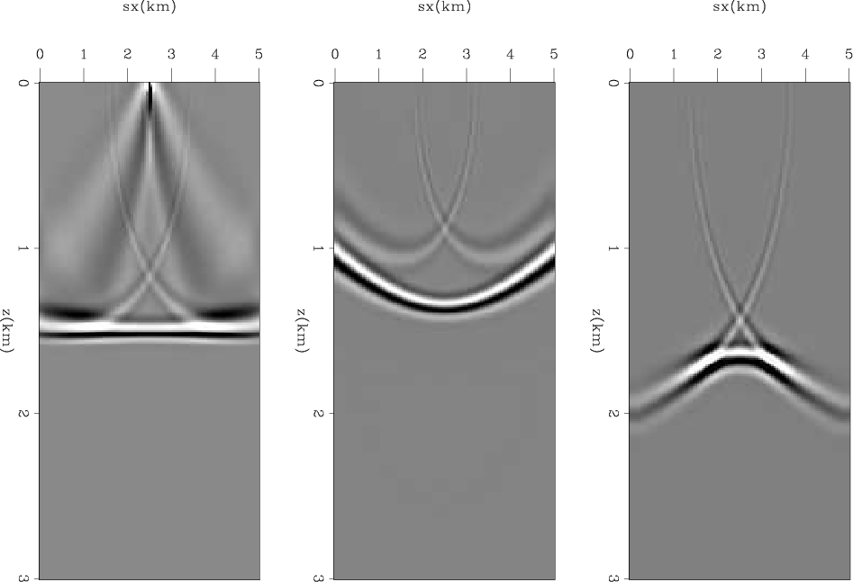
The extended inversion, whether in model space or data space, needs to satisfy two conditions. First, the observed data can always be explained by the extended model regardless of the selection of the initial model (Biondi, 2012). Second, the extended model should allow gradual change by regularization to produce a non-extended model. The data space extensions that can potentially satisfy these conditions are source location and source ray parameter. The source location extension has the advantage of using the exact same propagation engine as the conventional inversion, so its implementation requires minimal adjustment to existing applications. Moreover, the source location satisfies the extension conditions fairly well. Figure 1 shows source location image gathers for a two-layer model when using the correct velocity, a 10 percent lower velocity, and a 10 percent higher velocity. We see that regularizing the additional axis by a derivative can satisfy the second condition. The disadvantage of this extension is having a velocity model for each source location, which can require a very large memory size and burdensome I/O in 3D.

image-s Figure 1. Source location image gather for a two-layer model when using the correct velocity (left), a 10 percent lower velocity (middle), and a 10 percent higher velocity (right).

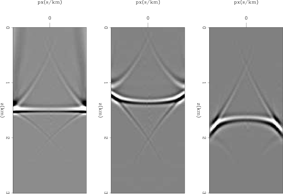
Extending the model by source ray parameter requires plane-wave encoding of the data (Whitmore, 1995; Liu et al., 2006; Zhang et al., 2005). Figure 2 shows source ray parameter image gathers for a two-layer model when using the correct velocity, a 10 percent lower velocity, and a 10 percent higher velocity. Similar to source location, the source ray parameter seems to also satisfy the second condition of model extension. The first condition is tested in the Synthetic Examples section below. In addition, the number of planes is generally much smaller than the number of source locations, so it both reduces the cost and makes the size of the extended model very manageable.

image-p Figure 2. Source ray parameter image gather for a two-layer model when using the correct velocity (left), a 10 percent lower velocity (middle), and a 10 percent higher velocity (right).

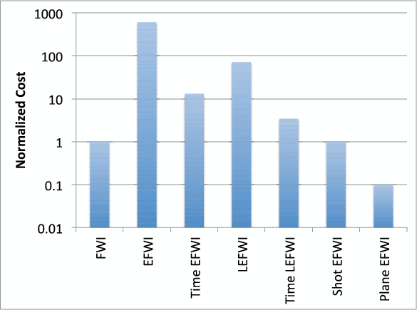
The cost of source location encoding is the same as conventional FWI, whereas the cost of source ray parameter extension is

$$C_{\rm Ray EFWI} = N_x N_y N_z N_p (6 \times N_{tp} C_{\rm FDTD} + 6 \times N_{tp} + N_{ti}),$$ (20)

where $N_p$ is the number of planes. Figure 3 compares the costs of all mentioned inversions assuming $N_x=N_y=1000$ , $N_z=100$ , $N_{\rm source}=10000$ , $C_{\rm FDTD}=16$ , $N_{tp}=1000$ , $N_{ti}=100$ , $N_{hx}=N_{hy}=100$ , $N_{\tau}=200$ , and $N_p=1000$ , where the costs are normalized by the cost of conventional FWI. The log-scale highlights that the difference in cost between these inversions can be several orders of magnitude.

CostEFWI Figure 3. Cost comparison of conventional and extended full wavefrom inversions.

Computational analysis of extended full waveform inversion