|
|
|
|
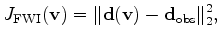
Single frequency 2D acoustic full waveform inversion |
 can be written as:
 is the velocity model,
 is the computed data, and
 is the observed data.
is computed as:
is the observed data.
is computed as:
 is the source function,
  is frequency,
 and
and
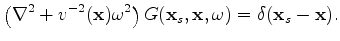
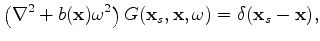
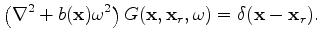
 are the source and receiver coordinates, and
  is the model coordinate. In the acoustic, constant-density case the Green's function
 satisfies:
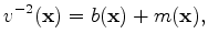
 is the background component, which is the current model in slowness squared units, and
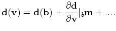
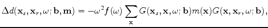
 is the perturbation component. After this separation, we can use Taylor expansion on the data around the background component as follows:
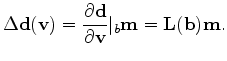
 as:
as:
 as follows:
 is the step size. To estimate the step size, we first evaluate the objective function with the gradient scaled to have a maximum of 2% and 4% of the minimum value of the current model. Using these two points as well as the objective function value at the current model, which is already computed in the gradient calculation, we fit a parabola. If the parabola has positive-side minimum, i.e. both the curvature and the x-axis shift are positive, a new objective function evaluation is performed at the parabola minimum. Then, the two or three evaluations are compared and the scale that resulted in the smallest objective function is used as the step size given that the objective function decreases. Otherwise, the line search is repeated after shrinking the gradient by a factor of 4. The optimization scheme is implemented on the CPU in Fourier domain notations using frequency domain Green's function solutions computed on the GPU.
|
|
|
|
Single frequency 2D acoustic full waveform inversion |