Single frequency 2D acoustic full waveform inversion

Introduction

Surface waves naturally propagate in two dimensions along the earth's surface and not in depth. However, du to their wavelength their waves' motion causes disturbances away from the interface, thus making surface waves sensitive to mechanical properties away from the interface. This is manifested in a variability of the wave propagation speed with frequency, i.e. dispersion. Dispersive Scholte waves can be extracted from ambient seismic noise by cross-correlation (de Ridder and Dellinger, 2011; de Ridder, 2012). Kimman (2011) found that higher modes are often not constructed or very weak, when the excitations are located at the surface. Furthermore, de Ridder (2012) shows how Scholte waves reconstructed from ambient seismic noise at Valhall field contain a single mode dispersive surface wave.

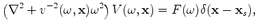
An approximate physical model for a single mode of surface waves is waves travelling in two dimensions given a phase velocity map, $c(\omega,\mathbf{x})$ . The amplitudes and phases of surface waves, in that approximation, are governed by

$$\left( \nabla^2 + v^{-2}(\omega,\mathbf{x})\omega^2 \right) V(\omega,\mathbf{x}) = F(\omega)\delta(\mathbf{x}-\mathbf{x}_s),$$ (1)

where $\mathbf{x}=(x,y)$ and $\nabla^2 = \partial_x^2 + \partial_y^2$ . Equation 1 is very similar to a classical 2D acoustic wave equation, except that the velocity is now a function of frequency. Explicitly solving for a single frequency renders this difference moot. However, frequency domain solutions are slow to compute, and implementation of absorbing boundary conditions is not straightforward. Here we solve equation 1 by a time-domain equivalent, valid for individual frequencies and independent of boundary condition.

We want to use equation 1 to image the phase-velocity cube $v(\omega,\mathbf{x})$ by full waveform inversion (FWI) for each frequency separately. But single frequency data generally does not resolve anomalies in space, because sensitivity kernels have endless oscillatory behaviour. Conventionally, summing over a finite frequency band collapses the sensitivity kernels to the classic and familiar banana-doughnut kernels (Dahlen and Nolet, 2000). However, in this paper we show that a similar effect is achieved by having sources and receivers throughout and around the target of interest.

This paper starts by connecting a time domain kernel to solutions of the 2D frequency domain acoustic kernels with frequency dependant velocity. Then a non-linear optimization algorithm is developed to invert single frequency amplitude and phase data. Finally we explore the ability of various acquisition grids to invert for a Gaussian anomaly.

Single frequency 2D acoustic full waveform inversion