Continuous monitoring by ambient-seismic noise tomography

Ambient seismic-seismic noise tomography

The virtual seismic sources are dominated by dispersive surface waves. These propagate in two dimensions along the seafloor through a frequency-dependent velocity map. Group velocities of the surface waves can be found for narrow frequency ranges. We use a simple Hann-window bandpass to select a narrow frequency range, and then we pick travel times by the maximum of the envelope of the filtered time-domain virtual-source arrival. We define a quality factor on each pick by a signal to noise ratio (SNR): the maximum of the envelope within a linear moveout window to the average of the envelope outside the window. For various narrow frequency bands we selected travel times, $\mathbf{t}$ , with an SNR $>$  5 and at offsets between $50$ and $1750$  meters. These travel-time picks were input into a straight-ray tomography kernel, linearized with perturbations, $\Delta \mathbf{m}$ , in an average velocity, $\mathrm{m}_0$ :

$$\mathbf{m} = \mathrm{m}_0 + \Delta \mathbf{m},$$ (2)

$$\mathrm{m}_0 = \frac{1}{N}\sum_{i=1}^{N} \frac{\mathbf{t}}{\Delta \mathbf{x}},$$ (3)

$$\Delta \mathbf{t} = \mathbf{t} - \mathrm{m}_0\ \Delta \mathbf{x},$$ (4)

where $\Delta \mathbf{t}$ are the travel-time residuals after accounting for the contribution of the average velocity and $\Delta \mathbf{x}$ is the offsets for each specific travel-time pick. The tomography-problem fitting goals are posed as follows:

$$\mathbf{F} \Delta \mathbf{m} - \Delta \mathbf{t} = \mathbf{0},$$ (5)

$$\epsilon \nabla^2 \Delta \mathbf{m} = \mathbf{0},$$ (6)

where we use the $\nabla^2$ operator as regularization to force a smooth model, and the total model is reconstructed by summing with the background velocity.

The aim is to create group-velocity maps at different frequencies by picking a group travel time at the peak of the envelope after a narrow-range bandpass. Lower-frequency group-velocity maps should reflect deeper structures, because at lower frequencies (and thus longer wavelengths), surface waves are sensitive to deeper structures. Picking a frequency range that is too narrow would result in an oscillatory wavelet and make travel-time picks less accurate. Figure 9 contains a set of inversion results using virtual sources of different frequency ranges. Six overlapping frequency ranges were selected: $0.15 - 0.75$  Hz, $0.35 - 0.95$  Hz, $0.55 - 1.15$  Hz, $0.75 - 1.35$  Hz, $0.95 - 1.55$  Hz and for $1.15 - 1.75$  Hz. At all ranges but the lowest, the wave-mode is very sharply defined in the dispersion image of Figure 5.

JZTomo-C1,JZTomo-C2,JZTomo-C3,JZTomo-C4,JZTomo-C5,JZTomo-C6
Figure 9. Tomography results for various frequency bands: $0.15 - 0.75$  Hz (a), $0.35 - 0.95$  Hz (b), $0.55 - 1.15$  Hz (c), $0.75 - 1.35$  Hz (d), $0.95 - 1.55$  Hz (e), and for $1.15 - 1.75$  Hz (f).

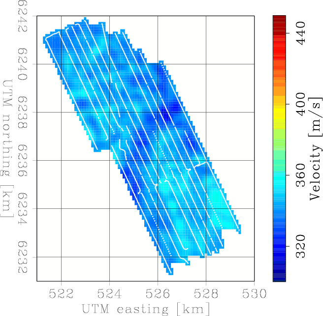
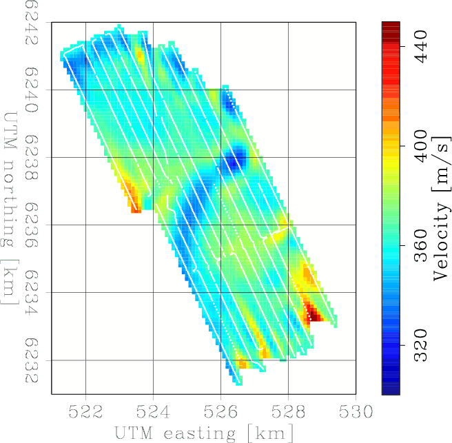
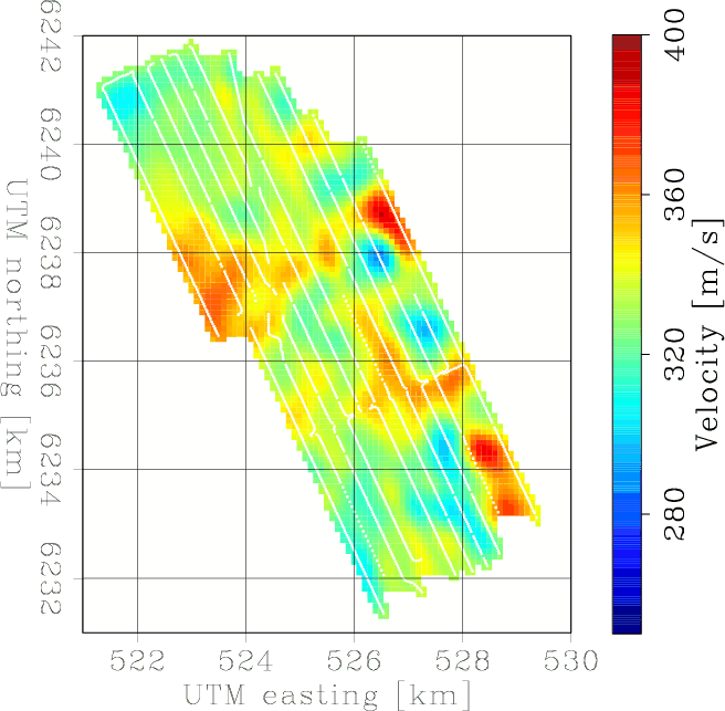
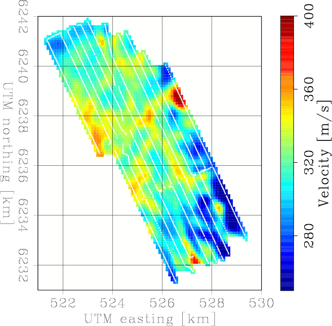
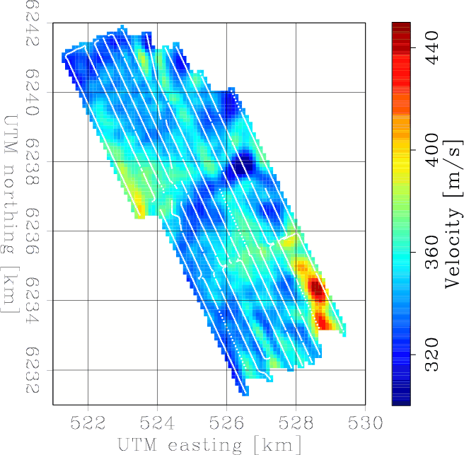
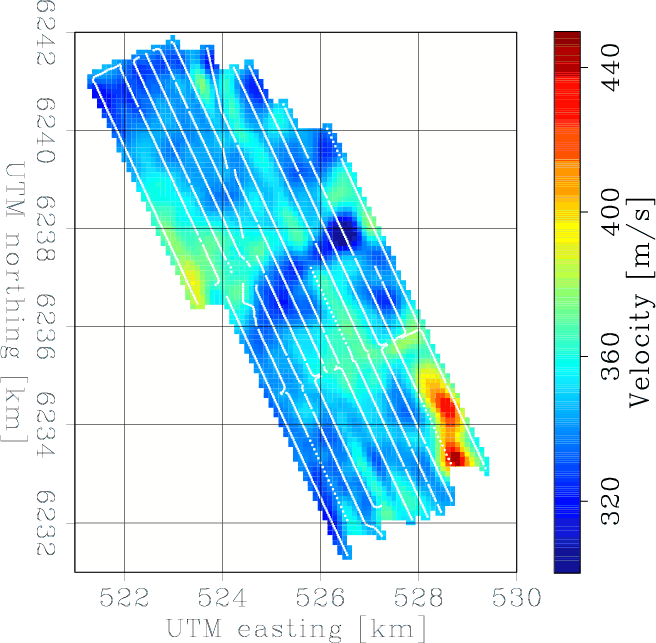
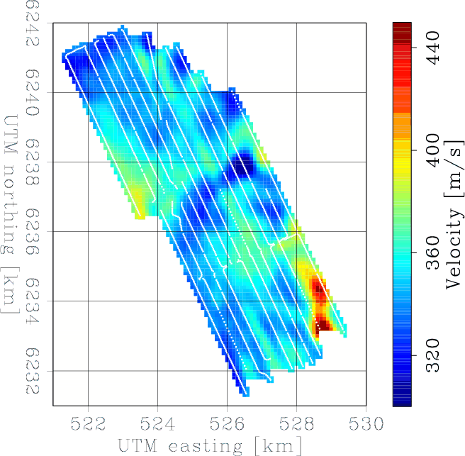
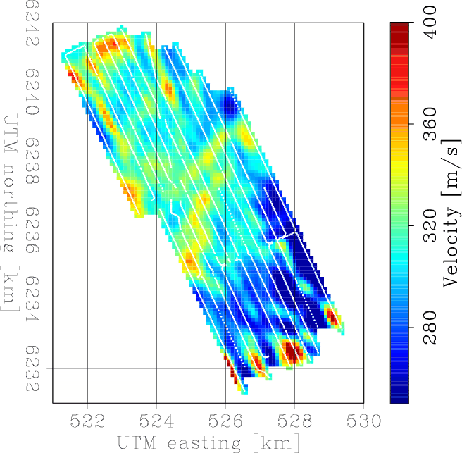
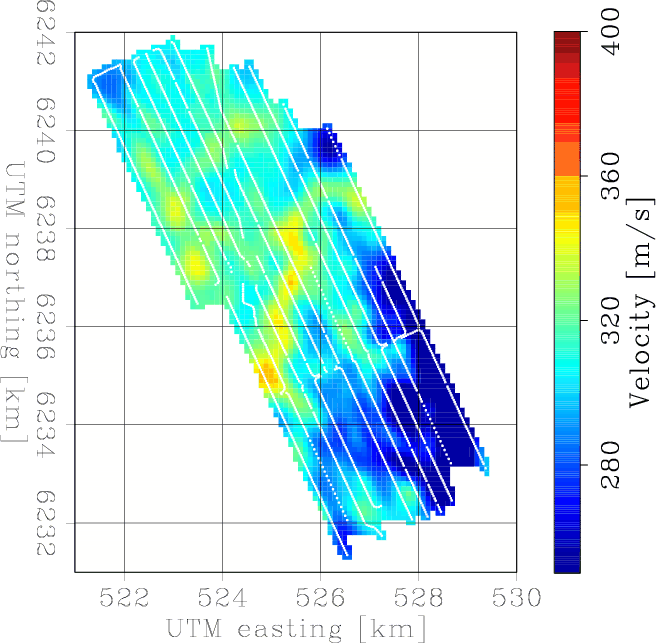
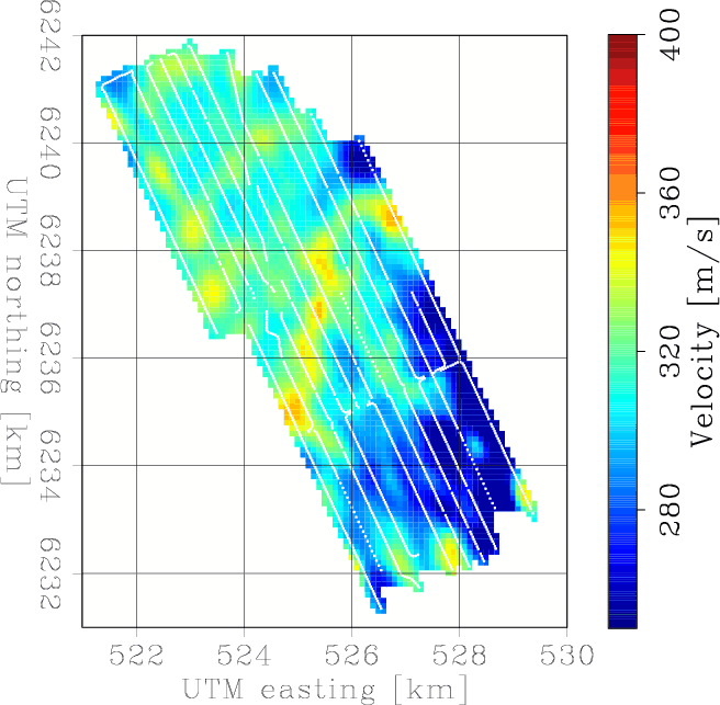
Stacking just one day of data gives five independent stacks. Five tomographic images, one for each day, of group-velocity for the frequency range $0.75 - 1.35$  Hz are shown in Figure 10. And five tomographic images, one for each day, of group-velocity for the frequency range $1.15 - 1.75$  Hz are shown in Figure 11. Stacking two and a half day of data gives two independent stacks. Four tomographic images, of both stacks, of group-velocity for the frequency ranges $0.75 - 1.35$  Hz and $1.15 - 1.75$  Hz are shown in Figure 12. These tomographic images are similar but not the same.

JZTomo-d1C3,JZTomo-d2C3,JZTomo-d3C3,JZTomo-d4C3,JZTomo-d5C3
Figure 10. Tomographic results for correlations of one day of data between $0.75 - 1.35$  Hz: day 1 (a), day 2 (b), day 3 (c), day 4 (d), day 5 (e).

JZTomo-d1C6,JZTomo-d2C6,JZTomo-d3C6,JZTomo-d4C6,JZTomo-d5C6
Figure 11. Tomographic results for correlations of one day of data between $1.15 - 1.75$  Hz: day 1 (a), day 2 (b), day 3 (c), day 4 (d), day 5 (e).

JZTomo-h1C3,JZTomo-h1C6,JZTomo-h2C3,JZTomo-h2C6
Figure 12. Tomographic results for correlations of two and a half days of data between $0.75 - 1.35$  Hz (a) and (c) and for correlations between $1.15 - 1.75$  Hz: from the first two and a half days in (a) and (b), from the second two and a half days in (b) and (d).

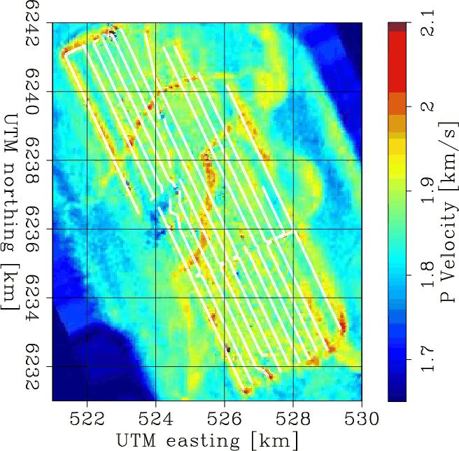
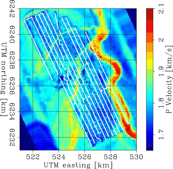
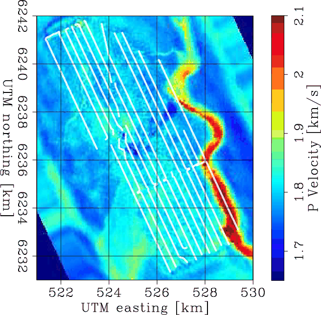
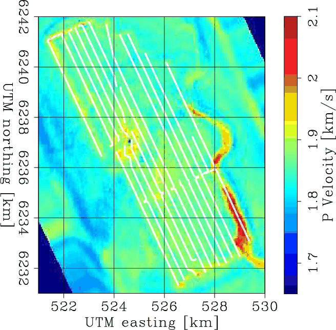
We can compare these group-velocity images to P-wave velocity images obtained by full wave-form inversion of active seismic surveys (Sirgue et al., 2010). These images include features extending beyond the extent of the receiver array, because the active sources cover a wider area than the receivers do. Whereas the maps obtained from ambient-seismic noise tomography are logically confined within the area of the recording array. In the $240$  meters below the seafloor, the P-wave velocity maps show several buried channels as high-velocity anomalies. The bigger channel on the east is as deep as $105$ to $240$  meters. There are smaller channels buried in the top $100$  meters. Below one of the smaller shallow channels is a low-velocity zone that crosses the array; this feature is apparent between $150$ and $240$  meters.

map3,map4,map5,map6
Figure 13. Image of P-wave velocities obtained using wave-form inversion of active P-wave data (Sirgue et al., 2010). Velocity slices are for the following depth ranges: $60 - 105$  m (a), $105 - 150$  m (b), $150 - 195$  m (c), and $195 - 240$  m (d).

Continuous monitoring by ambient-seismic noise tomography