Identifying reservoir depletion patterns from production-induced deformations with applications to seismic imaging

Estimating Pore-Pressure Decline from Displacements

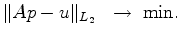
Denoting the operator in the right-hand side of equation 5 as $A$ , the problem of recovering the pore pressure decline from specified displacements can be cast as a least-squares minimisation problem:

$$\Vert Ap-u\Vert _{L_2}\ \; \rightarrow \; \textrm{min}.$$ (10)

To solve 10 we use the object-oriented Fortran 2003 optimisation framework exp_tk developed by the author that implements multiple general-purpose optimisation methods. The implementation is fully decoupled from underlying model and data structures and can be used in a variety of applications. The tools described in Appendix B implement forward modeling and inversion, with the latter performed by applying a Krylov solver (Trefethen and Bau, 1997),(Bjork, 1996) with a user-specified number of iterations.

pinvertedporeoutsymlowres,cinvertedporeoutsymlowres
Figure 4. a) Axisymmetric pore pressure decline inverted from the forward-modelled subsidence of Fig 2(b) on a sparse $11\times 11$ grid after 4 solver iterations. b) Contour plot of the inverted axisymmetric pore pressure of Fig 4(a).

We test the inversion code first by inverting the previously modelled displacement for the axisymmetric and asymmetric pore pressure decline patterns of of Fig 2(a) and 3(a). Fig 4(a) and Fig 4(b) show the result for the axisymmetric pore pressure decline inverted on a sparse $11\times 11$ grid in 4 iterations. We employ a multigrid approach (Iserles, 2008) where the inversion result obtained on a sparser grid is supplied as an initial approximation to the inversion on a denser grid. The inversion result for the $11\times 11$ grid was supplied as an initial approximation to the pressure decline for the inversion on the denser $81\times 81$ grid, and the resulting inverted axisymmetric pore pressure decline after 2 more iterations is shown on Fig 5(a) and Fig 5(b).

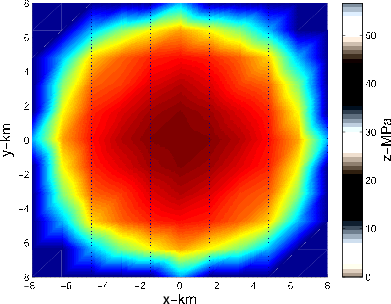
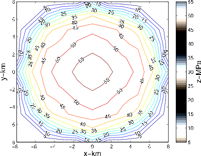
pinvertedporeoutsymhires,cinvertedporeoutsymhires
Figure 5. a) Axisymmetric pore pressure decline inverted from the forward-modelled subsidence of Fig 2(b) on a denser $81\times 81$ grid after 2 more solver iterations (total 6). b) Contour plot of the inverted axisymmetric pore pressure of Fig 5(a).

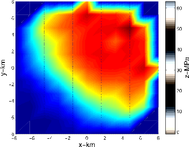
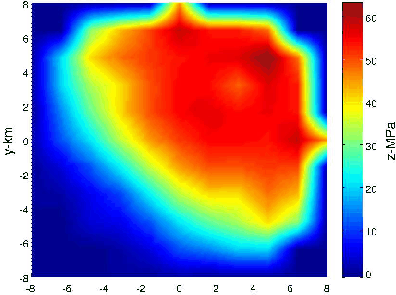
We have run a similar test for the asymmetric pore pressure decline of Fig 3(a) and equation 8. The result for the sparse grid and 5 iterations is shown on Fig 6(a) and Fig 6(b). The result of 2 more solver iterations on the denser grid is shown on Fig 7(a) and Fig 7(b).

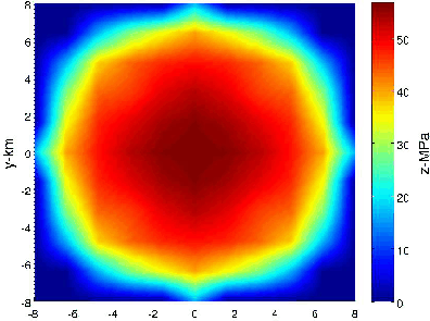
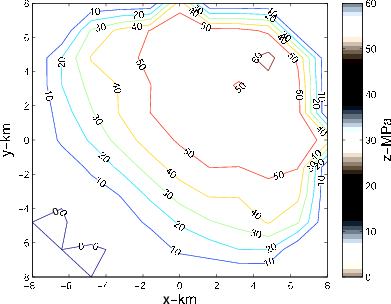
pinvertedporeoutasymlowres,cinvertedporeoutasymlowres
Figure 6. a) Asymmetric pore pressure decline inverted from the forward-modelled subsidence of Fig 3(b) on a sparse $11\times 11$ grid after 5 solver iterations. b) Contour plot of the inverted asymmetric pore pressure of Fig 6(a).

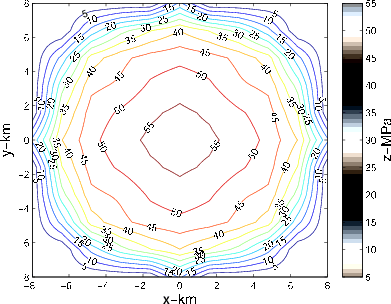
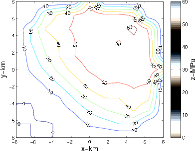
pinvertedporeoutasymhires,cinvertedporeoutasymhires
Figure 7. a) Asymmetric pore pressure decline inverted from the forward-modelled subsidence of Fig 3(b) on a denser $81\times 81$ grid after 2 more solver iterations (total 7). b) Contour plot of the inverted asymmetric pore pressure of Fig 7(a).

Comparison of Fig 5(b) with Fig 2(a) and of Fig 7(b) with Fig 3(a) indicates a good agreement of the inverted pore pressure decline with the synthetics, violated mostly by the distortions near reservoir edges. Due to the least-squares problem being ill-conditioned for large data and model spaces, convergence on denser reservoir grids cannot be achieved without a good initial approximation. This issue has been successfully resolved by using the multigrid approach.

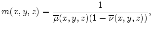
Note that although this test confirms the correct operation of our forward/inverse operator pair, by applying our inverse solver to the data modelled using the underlying forward-modeling operator we commit an inversion crime. True applicability of our method will be demonstrated in the next section where we apply it to a synthetic extrapolated from real subsidence data. While we are able to recover asymmetric pore pressure decline from as little data as can be contained in just one component of the measured displacement field, it is important to understand the sensitivity of our result to the uncertainty of the reservoir model parameters. Using operator 5 requires prior knowledge of medium and reservoir parameters, and using Mindlin's analytical expressions for elastostatic Green's tensor assumes homogeneity of the medium. In the numerical implementation of our method we effectively depart from the assumption of homogeneity by assuming instead local homogeneity or slow relative spatial change of medium parameters on the scales of reservoir length and depth. More precisely, our computational framework allows recasting operator 5 as

$$\mathbf{u}(x,y,z)\;=\;m(x,y,z)\mathbf{F}\left[r(\xi,\eta,\zeta) p(\xi,\eta,\zeta)\right]$$ (11)

where $\mathbf{F}$ is a homogeneous modeling operator, and $m(x,y,z)$ is a medium heterogeneity factor that, in the simplest case of slow-variability asymptotics (Maharramov, 2011),(Maslov, 1990),(Danilov et al., 1995), is equal to

$$m(x,y,z)=\frac{1}{\overline{\mu}(x,y,z)(1-\overline{\nu}(x,y,z))},$$ (12)

where the overscore in equation 12 represents some average value of the corresponding medium parameter. The scaler $r$ in the right-hand side of equation 11 is related to the heterogeneity of reservoir parameters, most notably the Biot coefficient. Equation 11 should include additional terms containing spatial derivatives of the Biot coefficient, but we ignore those terms under the assumption of mild spatial heterogeneity. Equation 11 suggests the following procedure for assessing the impact of the uncertainty in the values of the elastic moduli outside of the reservoir, assuming that $r$ in equation 11 is $1$ (i.e., reservoir parameters are integrated into $F$ ). The uncertainty of the pore pressure change due to a concentrated displacement $\delta(x-x_0,y-y_0,z-z_0)$ (along a fixed coordinate axis) is given by

$$\Delta p(\xi,\eta,\zeta)\;=\; \mathbf{F}^{-1}\left[ \delta (x,y,z)\right] \times \Delta \frac{1}{m(x_0,y_0,z_0)},$$ (13)

where the uncertainty $\Delta \frac{1}{m(x_0,y_0,z_0)}$ is computed from the associated uncertainties of the constituent medium parameters (e.g., moduli). Easy computation of the modeling operator and its inverse and the applicability of a multiscale/multigrid approach, as demonstrated in this paper, allow for a straightforward application of equation 13 to either estimating uncertainty or computing the mathematical expectation of the inverted pore pressure change.

Identifying reservoir depletion patterns from production-induced deformations with applications to seismic imaging