|
|
|
|
Decon in the log domain with variable gain |
We adopt the convention that components of a vector
 range over the values of
  , likewise for other vectors.
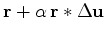
Given the gradient direction
, likewise for other vectors.
Given the gradient direction
 we need to know the residual change
 and a distance
  to go:
 and
and
 .
.
A two-term example demonstrates a required linearization.
 |
 |
 |
(18) |
|
|
 |
(19) |
 |
|
 |
(20) |
|
|
 |
(21) |
 ,
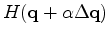
and knowing the gradient
,
let us work out the forward operator to find
,
and knowing the gradient
,
let us work out the forward operator to find
 .
Let ``
.
Let `` '' denote convolution.
is proportional to
'' denote convolution.
is proportional to
 .
This might mean we can deal with a wide dynamic range within
.
This might mean we can deal with a wide dynamic range within  .
The convolution, a physical process, occurs in the physical domain
which is only later gained to the statistical domain
.
The convolution, a physical process, occurs in the physical domain
which is only later gained to the statistical domain  .
Naturally, the convolution may be done as a product in the frequency domain.
.
Naturally, the convolution may be done as a product in the frequency domain.
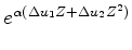
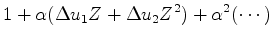
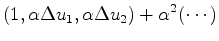
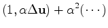
To minimize
 express it as a Taylor series approximation to quadratic order.
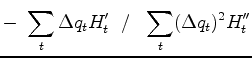
Minimizing yields
express it as a Taylor series approximation to quadratic order.
Minimizing yields
 |
|
 |
(29) |
 and
and
 ,
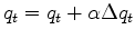
optionally (Newton method) iterate (because the locations of the many Taylor series
have changed slightly with the change in
,
optionally (Newton method) iterate (because the locations of the many Taylor series
have changed slightly with the change in
 ).
).
|
|
|
|
Decon in the log domain with variable gain |