VTI migration velocity analysis using RTM

Adjoint method from the perturbation theory

A perturbation, $\delta c$ , of the velocity model $c$ , induces a perturbation $\delta {\bf p}$ in the source wavefield vector ${\bf p}$ , a perturbation $\delta {\bf q}$ in the receiver wavefield vector ${\bf q}$ , a perturbation $\delta {\bf I}$ in the extended image cube ${\bf I}$ , and hence a perturbation $\delta J$ in the objective function $J$ . To the first order and using chain rule, $\delta J$ and $\delta c$ have following relationship:

$$\delta J = \sum_{\bf h} \frac{\partial J}{\partial I_{\bf h}} \fr... ...ial I_{\bf h}}{\partial {\bf q}} \frac{\partial {\bf q}}{\partial c} \delta c .$$ (16)

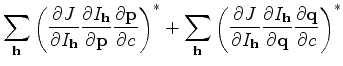
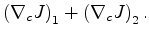
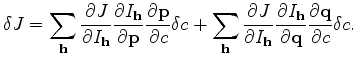
Now we can define the gradient by the back-projection of a unit perturbation in the objective function:

$$\nabla_c J = \sum_{\bf h}\left ( \frac{\partial J}{\partial I_{\bf h}} \frac{\... ...ial I_{\bf h}}{\partial {\bf q}} \frac{\partial {\bf q}}{\partial c} \right )^*$$

$$= \left(\nabla_c J\right)_1 + \left(\nabla_c J\right)_2.$$ (17)

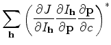
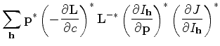
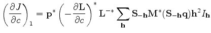
Let's analyze the first term in equation 17 in detail, and the second term follows the same reasoning.

$$\left(\nabla_c J\right)_1 = \sum_{\bf h} \left ( \frac{\partial J}{\partial I_{\bf h}} \frac{... ...ial I_{\bf h}}{\partial {\bf p}} \frac{\partial {\bf p}}{\partial c} \right )^*$$

$$= \sum_{\bf h} \left ( \frac{\partial {\bf p}}{\partial c} \right )... ...al {\bf p}} \right )^* \left ( \frac{\partial J}{\partial I_{\bf h}} \right )^*$$

$$= \sum_{\bf h} {\bf p}^* \left(-\frac{\partial {\bf L}}{\partial c}... ...\partial {\bf p}}\right)^* \left(\frac{\partial J}{\partial I_{\bf h}}\right)^*$$

$$= {\bf p}^* \left(-\frac{\partial {\bf L}}{\partial c}\right)^* {\b... ...\partial {\bf p}}\right)^* \left(\frac{\partial J}{\partial I_{\bf h}}\right)^*$$ (18)

where

$$\left ( \frac{\partial J}{\partial I_{\bf h}} \right )^* = {\bf h}^*{\bf h} I_{\bf h},$$ (19)

and

$$\left ( \frac{\partial I_{\bf h}}{\partial {\bf p}} \right )^* = ({\bf S}_{+{\bf h}})^* {\bf M}^*({\bf S}_{-{\bf h}} {\bf q})$$

$$= {\bf S}_{-{\bf h}} {\bf M}^*({\bf S}_{-{\bf h}} {\bf q}).$$ (20)

Plugging equation 19 and 20 into equation 18, we can rewrite equation 18 explicitly as follows:

$$\left(\frac{\partial J}{\partial c}\right)_1 = {\bf p}^* \left (-... ... h} {\bf S}_{-{\bf h}} {\bf M}^*({\bf S}_{-{\bf h}} {\bf q}) {\bf h}^2I_{\bf h}$$ (21)

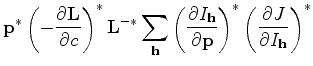
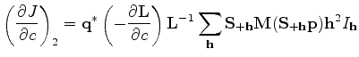
Similarly, we can obtain the explicit form for the second term in equation 17:

$$\left(\frac{\partial J}{\partial c}\right)_2 = {\bf q}^* \left (-... ...f h} {\bf S}_{+{\bf h}} {\bf M} ({\bf S}_{+{\bf h}} {\bf p}) {\bf h}^2I_{\bf h}$$ (22)

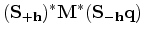
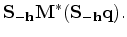
Substituting equation 21 and equation 22 for the corresponding terms in equation 17, we now have derived the explicit form for the DSO gradient.

VTI migration velocity analysis using RTM