|
|
|
|
Tomographic full waveform inversion: Practical and computationally feasible approach |
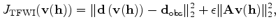
 which can be written as:
 is the offset,
 is the extended velocity model,
 is the modeled data,
 is the observed surface data,
  is a scalar weight of the regularization term and
  is a regularization operator. The modeled data
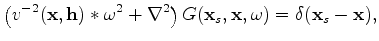
is computed as:
is a regularization operator. The modeled data
is computed as:
 is the source function,
  is frequency,
 and
and
 are the source and receiver coordinates, and
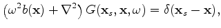
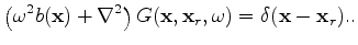
  is the model coordinate. In the acoustic, constant-density case the Green's function
 satisfies:
 denotes a convolution operator over the subsurface offset axis (Symes, 2008; Biondi and Almomin, 2012).
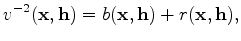
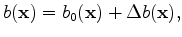
The first simplification of the extended velocity model is to separate it into a background and a perturbation as follows:
denotes a convolution operator over the subsurface offset axis (Symes, 2008; Biondi and Almomin, 2012).
The first simplification of the extended velocity model is to separate it into a background and a perturbation as follows:
 is the background component, which is a smooth version of the slowness squared and
 is the perturbation component. This separation assumes that
will contain the transmission effects and
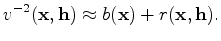
will contain the reflection effects. Depending on the error of the initial background velocity, the perturbation component can extend across several subsurface offsets so it is important to keep its offset axis. On the other hand, the background component is not expected to generate reflections that would be grossly time shifted with respect to the recorded data, and it thus safe to restrict it to zero offset. A physical interpretation is that the wave speed is not expected to vary much across different angles, at least in the isotropic case that we are analyzing. Therefore, the extent of background component across subsurface offsets can be reduced. If the velocity is expected to vary, the same reduction can be applied while keeping more than zero subsurface offset. In our derivation, we reduce the background to only the zero subsurface offset as follows
is the perturbation component. This separation assumes that
will contain the transmission effects and
will contain the reflection effects. Depending on the error of the initial background velocity, the perturbation component can extend across several subsurface offsets so it is important to keep its offset axis. On the other hand, the background component is not expected to generate reflections that would be grossly time shifted with respect to the recorded data, and it thus safe to restrict it to zero offset. A physical interpretation is that the wave speed is not expected to vary much across different angles, at least in the isotropic case that we are analyzing. Therefore, the extent of background component across subsurface offsets can be reduced. If the velocity is expected to vary, the same reduction can be applied while keeping more than zero subsurface offset. In our derivation, we reduce the background to only the zero subsurface offset as follows
 is the Born modeling operator. We now define a new objective function for the efficient TFWI inversion as:
 is the current background model and
 is the perturbation of the background. The Born approximation is used again to linearize the
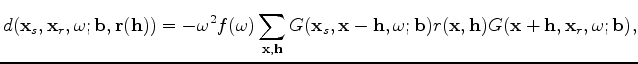
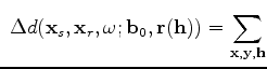
operator with respect to the background resulting in a data-space tomographic operator. The data perturbation with respect to the background perturbation is now defined as:
is the perturbation of the background. The Born approximation is used again to linearize the
operator with respect to the background resulting in a data-space tomographic operator. The data perturbation with respect to the background perturbation is now defined as:
 is the perturbation coordinates.
As we can see in the previous equation, the tomographic operator correlates a background and a scattered wavefield from both source and receiver sides. The scattered wavefields are computed by correlating a background wavefield with the reflectivity model
is the perturbation coordinates.
As we can see in the previous equation, the tomographic operator correlates a background and a scattered wavefield from both source and receiver sides. The scattered wavefields are computed by correlating a background wavefield with the reflectivity model  and then propagating again to all model locations.
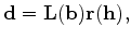
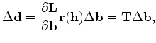
The forward tomographic operator can be written in a compact notation as follows:
and then propagating again to all model locations.
The forward tomographic operator can be written in a compact notation as follows:
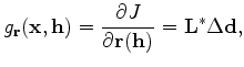
 is the tomographic operator that relates changes in the background model to changes in the data. We can now compute the reflectivity gradient as follows:
|
|
|
|
Tomographic full waveform inversion: Practical and computationally feasible approach |