Next: Dispersion relations
Up: WAVE-EXTRAPOLATION EQUATIONS
Previous: Meet the parabolic wave
Muir's method of finding wave extrapolators
seeks polynomial ratio approximations
to a square-root dispersion relation.
Then fractions are cleared
and the approximate dispersion relation is inverse transformed
into a differential equation.
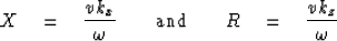
Substitution of the plane wave
 into the two-dimensional scalar wave equation (
![[*]](http://sepwww.stanford.edu/latex2html/cross_ref_motif.gif) )
yields the dispersion relation
)
yields the dispersion relation
|  |
(7) |
Solve for kz selecting the positive square root
(thus for the moment selecting
downgoing
waves).
| 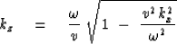 |
(8) |
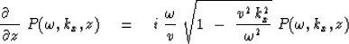
To inverse transform the z-axis we
only need to recognize that i kz corresponds
to  .The resulting expression is a wavefield extrapolator, namely,
|  |
(9) |
Bringing equation (9) into the space domain
is not simply a matter of substituting
a second x derivative for kx2.
The problem is the meaning of the square root of a differential operator.
The square root of a differential operator is not defined in
undergraduate calculus courses and there is no straightforward
finite difference representation.
The square root becomes meaningful only when the square root is regarded
as some kind of truncated series expansion.
It will be shown in chapter
that the Taylor series is a poor choice.
Francis Muir showed that my original 15 and 45 methods were
just truncations of a continued fraction expansion.
To see this, define
and 45 methods were
just truncations of a continued fraction expansion.
To see this, define
|  |
(10) |
So equation (8) is more simply and abstractly written as
|  |
(11) |
which you recognize as meaning that cosine
is the square root of one minus sine squared.
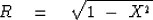
The desired polynomial ratio of order n will be
denoted Rn, and
it will be determined by the recurrence
|  |
(12) |
The recurrence is a guess
that we verify by seeing what it converges to (if it converges).
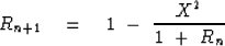
Set  in (12) and solve
|  |
|
| |
| (13) |
The square root of (13)
gives the required expression (11).
Geometrically, (13) says that the cosine squared of the incident
angle equals one minus the sine squared and
truncating the expansion leads to angle errors.
Muir said,
and you can verify,
that his recurrance relationship formalizes
what I was doing
by re-estimating the  term.
Although it is pleasing to think of large values of n,
in real life
only the low-order terms in the expansion are used.
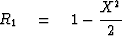
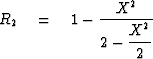
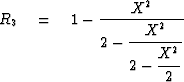
Table .1 shows the result of three Muir iterations
beginning from R0 = 1
term.
Although it is pleasing to think of large values of n,
in real life
only the low-order terms in the expansion are used.
Table .1 shows the result of three Muir iterations
beginning from R0 = 1
Table 1:
First four truncations of Muir's continued fraction expansion.
| |
|
 |
 |
| |
|
| |
|
 |
 |
| |
|
| |
|
 |
 |
| |
|
| |
|
 |
 |
| |
|
For various historical reasons,
the equations in Table .1 are often referred to as the
5, 15, and 45 equations, respectively,
the names giving a reasonable qualitative (but poor quantitative) guide to
the range of angles that are adequately handled.
A trade-off between complexity and accuracy frequently dictates choice of
the 45 equation.
It then turns out that a slightly wider range of angles can be
accommodated if the recurrence is begun
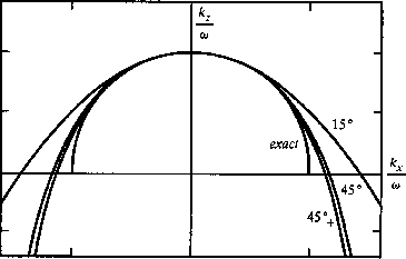
with something like  45.Figure 1 shows some plots.
disper
Figure 1
Dispersion relation of Table .2.
The curve labeled  was constructed
with
was constructed
with  .
It fits exactly at 0 and 45 .
.
It fits exactly at 0 and 45 .

Next: Dispersion relations
Up: WAVE-EXTRAPOLATION EQUATIONS
Previous: Meet the parabolic wave
Stanford Exploration Project
10/31/1997