


The Grand Isle data is incomprehensible in terms of the model based on layered media theory. Kjartansson proposed an alternative model. Figure 7 illustrates a geometry in which rays travel in straight lines from any source to a flat horizontal reflector, and thence to the receivers.
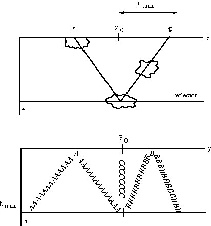 |

The only complications are ``pods'' of some material that is presumed to disturb seismic rays in some anomalous way. Initially you may imagine that the pods absorb wave energy. (In the end it will be unclear whether the disturbance results from energy focusing or absorbing).
Pod A is near the surface.
The seismic survey is affected by it twice--once
when the pod is traversed by the shot and once when it is
traversed by the geophone.
Pod C is near the reflector and encompasses a small area of it.
Pod C is seen at all offsets h but only at one midpoint, y0.
The raypath depicted on the top of Figure 7 is one that is
affected by all pods.
It is at midpoint y0 and at the widest offset ![]() .Find the raypath on the lower diagram in Figure 7.
.Find the raypath on the lower diagram in Figure 7.
Pod B is part way between A and C. The slope of affected points in the (y,h)-plane is part way between the slope of A and the slope of C.
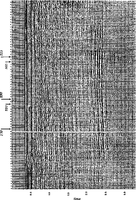
Figure 8 shows a common-offset section across the gas field. The offset shown is the fifth trace from the near offset, 1070 feet from the shot point. Don't be tricked into thinking the water was deep. The first break at about .33 seconds is wide-angle propagation.
 |
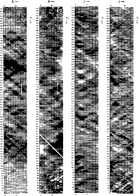 |
The power in each seismogram was computed in the interval from
1.5 to 3 seconds.
The logarithm of the power is plotted in Figure 9a as a function
of midpoint and offset.
Notice streaks of energy slicing across the (y,h)-plane
at about a 45![]() angle.
The strongest streak crosses at exactly 45
angle.
The strongest streak crosses at exactly 45![]() through the near offset at shot point 170.
This is a missing shot, as is clearly visible in Figure 8.
Next, think about the gas sand described as pod C in the model.
Any gas-sand effect in the data should show up as a streak
across all offsets at the midpoint of the gas sand--that is,
horizontally across the page.
I don't see such streaks in Figure 9a.
Careful study of the figure shows that
the rest of the many clearly visible streaks cut the plane at
an angle noticeably
less
than
through the near offset at shot point 170.
This is a missing shot, as is clearly visible in Figure 8.
Next, think about the gas sand described as pod C in the model.
Any gas-sand effect in the data should show up as a streak
across all offsets at the midpoint of the gas sand--that is,
horizontally across the page.
I don't see such streaks in Figure 9a.
Careful study of the figure shows that
the rest of the many clearly visible streaks cut the plane at
an angle noticeably
less
than ![]() 45
45![]() .The explanation for the angle of the streaks in the figure
is that they are like pod B.
They are part way between the surface and the reflector.
The angle determines the depth.
Being closer to 45
.The explanation for the angle of the streaks in the figure
is that they are like pod B.
They are part way between the surface and the reflector.
The angle determines the depth.
Being closer to 45![]() than to 0
than to 0![]() , the pods are
closer to the surface than to the reflector.
, the pods are
closer to the surface than to the reflector.
Figure 9b shows timing information in the same form that Figure 9a shows amplitude. A CDP stack was computed, and each field seismogram was compared to it. A residual time shift for each trace was determined and plotted in Figure 9b. The timing residuals on one of the common-midpoint gathers is shown in Figure 10.
|
kjmid
Figure 10 Midpoint gather 220 (same as timing of (h,y) in Figure 9b) after moveout. Shown is a one-second window centered at 2.3 seconds, time shifted according to an NMO for an event at 2.3 seconds, using a velocity of 7000 feet/sec. (Kjartansson) | 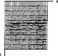 |
The results resemble the amplitudes, except that the results become noisy when the amplitude is low or where a ``leg jump'' has confounded the measurement. Figure 9b clearly shows that the disturbing influence on timing occurs at the same depth as that which disturbs amplitudes.
The process of inverse slant stack , to be described in Section 5.2 enables us to determine the depth distribution of the pods. This distribution is displayed in figures 9c and 9d.