Viscosity and causality

The frequency $\omega$ will range over $\pm \pi / \Delta t$.If the t-axis is going to be handled by finite differencing then we will need the Z-transform variable equation (50)  

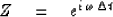$$Z \eq e^{{i} \, \omega \, \Delta t}$$ (50)

and the causal derivative (52)  

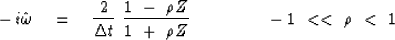$$- \, i \hat \omega \eq { {2 \over \Delta t } \ { 1 \ -\ \rh... ... +\ \rho Z } } \ \ \ \ \ \ \ \ \ \ \ \ \ -1 \ << \ \rho \ < \ 1$$ (51)

The data can be subsampled or supersampled before processing, so $\Delta t$ is an adjustable parameter. The causality parameter $\rho$ should be a small amount less than unity, say $\rho=1-\epsilon$ where $\epsilon \gt 0$ is an adjustable parameter. You may want to introduce $\rho$ even if you are migrating in the frequency domain because it reduces wraparound in the time domain--it is a kind of viscosity. The $\epsilon$ should be about inverse to the data length, say 1 / N_t where N_t is the number of points on the time axis. (Because I made many plots of synthetic hyperbolas with square root gain, $\gamma =1/2$, time wraparounds were larger than life. So I had the program default to $\epsilon$ four times larger). If you like to adjust free parameters, you could separately adjust numerator and denominator values of $\rho$.Subsequently, I'll distinguish between $\omega$ and $\hat \omega$,but you can take $\hat \omega$ to be $\omega$ if you don't care to introduce causality.