BLIND DECONVOLUTION

The prediction-error filter solves the ``blind-deconvolution'' problem. So far little has been said about the input data to the PE filter. A basic underlying model is that the input data results from white noise into a filter, where the filter is some process in nature. Since the output of the PE filter is white, it has the same spectrum as the original white noise. The natural hypothesis is that the filter in nature is the inverse of our PE filter. Both filters are causal, and their amplitude spectra are mutually inverse. Theoretically, if the model filter were minimum phase, then its inverse would be causal, and it would be our PE filter. But if the model filter were an all-pass filter, or had an all-pass filter as a factor, then its inverse would not be causal, so it could not be our PE filter.

 

model Figure 11 Spectra of random numbers, a filter, and the output of the filter.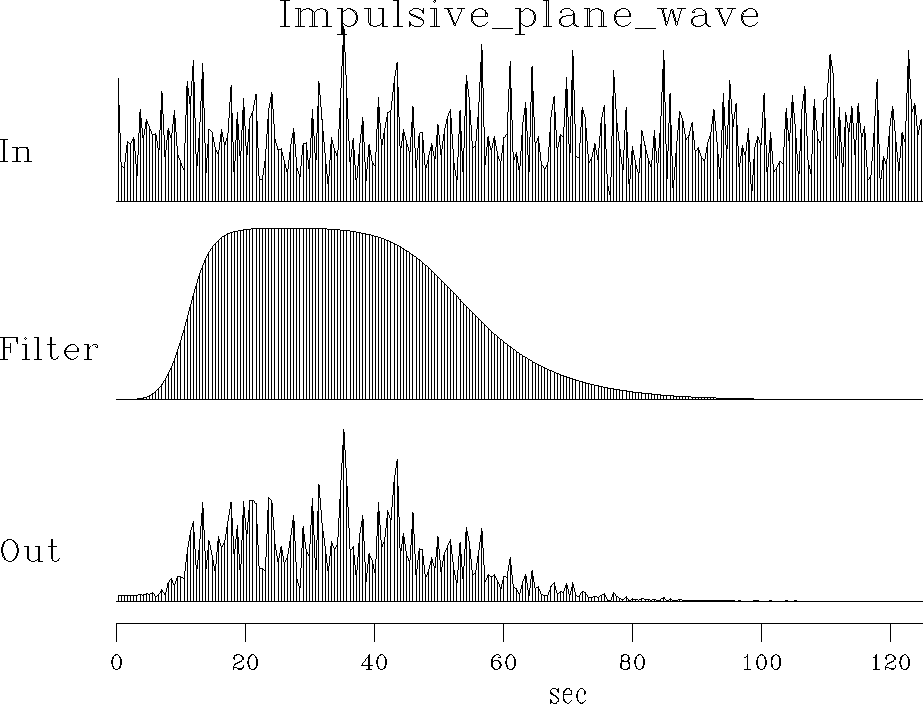

The blind-deconvolution problem can be attacked without PE filters by going to the frequency domain. Figure 11 shows sample spectra for the basic model. We see that the spectra of the random noise are random-looking. In chapter we will study random noise more thoroughly; the basic fact important here is that the longer the random time signal is, the rougher is its spectrum. This applies to both the input and the output of the filter. Smoothing the very rough spectrum of the input makes it tend to a constant; hence the common oversimplification that the spectrum of random noise is a constant. Since for Y(Z)=F(Z)X(Z) we have $\vert Y(\omega )\vert=\vert F(\omega )\vert\vert X(\omega )\vert$,the spectrum of the output of random noise into a filter is like the spectrum of the filter, but the output spectrum is jagged because of the noise. To estimate the spectrum of the filter in nature, we begin with data (like the output in Figure 11) and smooth its spectrum, getting an approximation to that of the filter. For blind deconvolution we simply apply the inverse filter.

The simplest way to get such a filter is to inverse transform the smoothed amplitude spectrum of the data to a time function. This time-domain wavelet will be a symmetrical signal, but in real life the wavelet should be causal. Chapter shows a Fourier method, called the ``Kolmogoroff method," for finding a causal wavelet of a given spectrum. Chapter shows that the length of the Kolmogoroff wavelet depends on the amount of spectral smoothing, which in this chapter is like the ratio of the data length to the filter length.

In blind deconvolution, Fourier methods determine the spectrum of the unknown wavelet. They seem unable to determine the wavelet's phase by measurements, however--only to assert it by theory. We will see that this is a limitation of the ``stationarity'' assumption, that signal strengths are uniform in time. Where signal strengths are nonuniform, better results can be found with weighting functions and time-domain methods. In Figure 14 we will see that the all-pass filter again becomes visible when we take the trouble to apply appropriate weights.