

Next: Solving tridiagonal simultaneous equations
Up: FINITE DIFFERENCING
Previous: The leapfrog method
The Crank-Nicolson method solves both the accuracy and the
stability problem.
Recall the difference representation of the heat-flow equation (32).
|  |
(34) |
Now, instead of expressing the right-hand side entirely at time t,
it will be averaged at t and t+1, giving
| ![\begin{displaymath}
q_{{t+1}}^x - q_t^x \eq {a \over 2 }\left[
\left( q_t^{{x+1}...
...}^{{x+1}} - 2q_{{t+1}}^x + q_{{t+1}}^{{x-1}} \right) \, \right]\end{displaymath}](img98.gif) |
(35) |
This is called the Crank-Nicolson method.
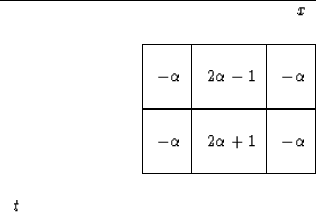
Defining a new parameter
 ,the difference star is
|  |
(36) |
When placing this star over the data table, note that,
typically, three elements at a time cover unknowns.
To say the same thing with equations,
move all the t+1 terms in
(35) to the left and the t terms to the right, obtaining
|  |
(37) |
Now think of the left side of equation (37)
as containing all the unknown quantities
and the right side as containing all known quantities.
Everything on the right can be combined into a single known quantity,
say, dtx.
Now we can rewrite equation (37)
as a set of simultaneous equations.
For definiteness,
take the x-axis to be limited to five points.
Then these equations are:
| ![\begin{displaymath}
\left[
\matrix {
\matrix { e_{\rm left} \cr - B\cr 0 \cr 0 \...
...rix {
d_t^1 \cr d_t^2 \cr d_t^3 \cr d_t^4 \cr d_t^5 }
}
\right]\end{displaymath}](img102.gif) |
(38) |
Equation (37)
does not give us each  explicitly, but
equation (38)
gives them
implicitly
by the solution of simultaneous equations.
The values  and
and  are adjustable
and have to do with the side boundary conditions.
The important thing to notice is that the matrix is tridiagonal, that is,
except for three central diagonals all the elements of the
matrix in (38) are zero.
The solution to such a set of simultaneous equations
may be economically obtained.
It turns out that the cost is only about twice
that of the explicit method given by (32).
In fact, this implicit method turns out to
be cheaper, since the increased accuracy
of (37) over (32)
allows the use of a much larger numerical choice
of
  .A program that demonstrates the stability of the method,
even for large
  , is given next.
A tridiagonal simultaneous equation
solving subroutine rtris() explained in the next section.
The results are stable, as you can see.
a = 8.00
  0.00  0.00  0.00  0.00  0.00  0.00  1.00  1.00  1.00  1.00  1.00  1.00
  0.17  0.17  0.21  0.30  0.47  0.76  0.24  0.53  0.70  0.79  0.83  0.83
  0.40  0.40  0.42  0.43  0.40  0.24  0.76  0.60  0.57  0.58  0.60  0.60
  0.44  0.44  0.44  0.44  0.48  0.68  0.32  0.52  0.56  0.56  0.56  0.56
# Implicit heat-flow equation
real q(12),d(12)
nx=12; a = 8.;	write(6,'(/"a =",f5.2)') a;	alpha = .5*a
do ix= 1,6  {	q(ix) = 0.}	# Initial temperature step
do ix= 7,12 {	q(ix) = 1.}
do it= 1,4 {
	write(6,'(20f6.2)') (q(ix),ix=1,nx)
	d(1) = 0.;	d(nx) = 0.
	do ix= 2, nx-1
		d(ix) = q(ix) + alpha*(q(ix-1)-2.*q(ix)+q(ix+1))
	call rtris( nx, alpha, -alpha, (1.+2.*alpha), -alpha, alpha, d, q)
	}
call exit(0);	end


Next: Solving tridiagonal simultaneous equations
Up: FINITE DIFFERENCING
Previous: The leapfrog method
Stanford Exploration Project
10/31/1997

![\begin{displaymath}
\left[
\matrix {
\matrix { e_{\rm left} \cr - B\cr 0 \cr 0 \...
...rix {
d_t^1 \cr d_t^2 \cr d_t^3 \cr d_t^4 \cr d_t^5 }
}
\right]\end{displaymath}](img102.gif)
![]() and
and ![]() are adjustable
and have to do with the side boundary conditions.
The important thing to notice is that the matrix is tridiagonal, that is,
except for three central diagonals all the elements of the
matrix in (38) are zero.
The solution to such a set of simultaneous equations
may be economically obtained.
It turns out that the cost is only about twice
that of the explicit method given by (32).
In fact, this implicit method turns out to
be cheaper, since the increased accuracy
of (37) over (32)
allows the use of a much larger numerical choice
of
are adjustable
and have to do with the side boundary conditions.
The important thing to notice is that the matrix is tridiagonal, that is,
except for three central diagonals all the elements of the
matrix in (38) are zero.
The solution to such a set of simultaneous equations
may be economically obtained.
It turns out that the cost is only about twice
that of the explicit method given by (32).
In fact, this implicit method turns out to
be cheaper, since the increased accuracy
of (37) over (32)
allows the use of a much larger numerical choice
of ![]() .A program that demonstrates the stability of the method,
even for large
.A program that demonstrates the stability of the method,
even for large ![]() , is given next.
, is given next.